3  NOAA Fisheries recreational landings data

Here we will partition recreational landings data from NOAA Fisheries’ Marine Recreational Information Program (MRIP), a standardized, peer-reviewed suite of recreational fishing surveys used to produce catch and effort estimates for quota monitoring and stock assessment in the United States. MRIP is a standardized survey suite that employs a complex statistical sampling design stratified across time, regions of the coast, and different fishing modes, which allows the intercept data to be scaled up by effort estimates to calculate total catches.

3.1 Data access and upload

Data are downloaded directly from the Miami server using the files provided to SERO for ACL monitoring. The current location is: M://SFD/SECM-SFD/ACL/2025_Jun23_MRIP_MRFSS/. The landings are in FES MRIP and the units are in pounds whole weight.

# clear workspace
rm(list = ls())

# read in data file
load("data/mrip_fes_rec81_25wv2_23June25.RData")  # most recent file on SFD server
head(dat)
  REC_ACL_MRIP_FES_ID YEAR MONTH WAVE SUB_REG NEW_ST NEW_STA NEW_MODE NEW_MODEN
1            73407425 1989    NA    4       6      9      NC        4      Priv
2            73407426 1989    NA    4       6      9      NC        4      Priv
3            73407427 1989    NA    4       6      9      NC        4      Priv
4            73407428 1989    NA    4       6      9      NC        4      Priv
5            73407429 1989    NA    4       6      9      NC        4      Priv
6            73407430 1989    NA    4       6      9      NC        4      Priv
  AREA_X NEW_AREA  NEW_AREAN FL_REG NC_REG   DS               NEW_SCI
1      5        5    Inshore     NA      S MRIP Centropristis striata
2      5        5    Inshore     NA      N MRIP Centropristis striata
3      2        2  Ocean>3mi     NA      N MRIP Centropristis striata
4      2        2  Ocean>3mi     NA      S MRIP Centropristis striata
5      1        1 Ocean<=3mi     NA      N MRIP Centropristis striata
6      1        1 Ocean<=3mi     NA      S MRIP Centropristis striata
         NEW_COM    SP_CODE SPECIES_ITIS SPECIES        AB1          B2
1 black sea bass 8835020301       167687         34181.4033 121019.1368
2 black sea bass 8835020301       167687           795.8612   4445.0527
3 black sea bass 8835020301       167687           549.5390   2919.4840
4 black sea bass 8835020301       167687         71823.2390  24548.2535
5 black sea bass 8835020301       167687           415.7642     87.5928
6 black sea bass 8835020301       167687         48728.5632  11859.6428
           A         B1 LBSEST_SECWWT LBSEST_SECSOURCE SAMPLE_SIZE_USED
1 31761.4755  2419.9278    11457.8425          srysmwa               41
2   584.4155   211.4457      266.7782          srysmwa               41
3   549.5390     0.0000      484.4319          srysmwa              119
4 33343.1844 38480.0546    63313.9276          srysmwa              119
5   415.7642     0.0000      294.0623          srysmwa               71
6 40585.0152  8143.5480    34464.8156          srysmwa               71
   AVG_LEN   AVG_WGT SRYSMWA_AVG_LEN SRYSMWA_AVG_WGT SRYSMWA_SAMPLE_SIZE
1 203.4572 0.3352069        203.4572       0.3352069                  41
2 203.4572 0.3352069        203.4572       0.3352069                  41
3 296.2590 0.8815243        296.2590       0.8815243                 119
4 296.2590 0.8815243        296.2590       0.8815243                 119
5 261.9949 0.7072816        261.9949       0.7072816                  71
6 261.9949 0.7072816        261.9949       0.7072816                  71
  SRYSMWA_FLAGGED SRYSMW_AVG_LEN SRYSMW_AVG_WGT SRYSMW_SAMPLE_SIZE
1              NA       269.2563      0.7310037                231
2              NA       269.2563      0.7310037                231
3              NA       269.2563      0.7310037                231
4              NA       269.2563      0.7310037                231
5              NA       269.2563      0.7310037                231
6              NA       269.2563      0.7310037                231
  SRYSMW_FLAGGED SRYSM_AVG_LEN SRYSM_AVG_WGT SRYSM_SAMPLE_SIZE SRYSM_FLAGGED
1             NA      259.7694     0.6948228               556            NA
2             NA      259.7694     0.6948228               556            NA
3             NA      259.7694     0.6948228               556            NA
4             NA      259.7694     0.6948228               556            NA
5             NA      259.7694     0.6948228               556            NA
6             NA      259.7694     0.6948228               556            NA
  SRYS_AVG_LEN SRYS_AVG_WGT SRYS_SAMPLE_SIZE SRYS_FLAGGED SRY_AVG_LEN
1      270.955    0.8099641              982           NA    269.1276
2      270.955    0.8099641              982           NA    269.1276
3      270.955    0.8099641              982           NA    269.1276
4      270.955    0.8099641              982           NA    269.1276
5      270.955    0.8099641              982           NA    269.1276
6      270.955    0.8099641              982           NA    269.1276
  SRY_AVG_WGT SRY_SAMPLE_SIZE SRY_FLAGGED SR_AVG_LEN SR_AVG_WGT SR_SAMPLE_SIZE
1   0.8085211            1703          NA   303.6871   1.050403          46055
2   0.8085211            1703          NA   303.6871   1.050403          46055
3   0.8085211            1703          NA   303.6871   1.050403          46055
4   0.8085211            1703          NA   303.6871   1.050403          46055
5   0.8085211            1703          NA   303.6871   1.050403          46055
6   0.8085211            1703          NA   303.6871   1.050403          46055
  SR_FLAGGED S_AVG_LEN S_AVG_WGT S_SAMPLE_SIZE S_FLAGGED     VAR_B2   VAR_AB1
1         NA  344.4373  1.364082        305089        NA 4072492794 310099094
2         NA  344.4373  1.364082        305089        NA    2866289    258947
3         NA  344.4373  1.364082        305089        NA          0         0
4         NA  344.4373  1.364082        305089        NA  105731413 534702898
5         NA  344.4373  1.364082        305089        NA          0         0
6         NA  344.4373  1.364082        305089        NA   22265768 286196169
         SA_LABEL GOM_LABEL REC_ACL MIGRA_GRP AGG_MODEN JURISDICTION PS_REG
1 Snapper Grouper                 1             Private        State      6
2 Snapper Grouper                 1             Private        State      5
3 Snapper Grouper                 1             Private      Federal      5
4 Snapper Grouper                 1             Private      Federal      6
5 Snapper Grouper                 1             Private        State      5
6 Snapper Grouper                 1             Private        State      6
  COUNCILREG GFMC_FMP SAFMC_FMU LBSEST_SECGWT AGGR_AREA AREA FIRST_MONTH
1          6                  Y     9710.0360             NA          NA
2          5                  Y      226.0832             NA          NA
3          5                  Y      410.5355             NA          NA
4          6                  Y    53655.8708             NA          NA
5          5                  Y      249.2054             NA          NA
6          6                  Y    29207.4709             NA          NA
  LAST_MONTH ALT_FLAG CHTS_CL CHTS_H CHTS_RL CHTS_WAB1C CHTS_WAB1H MODE_FX
1         NA        0       0      0       0          0          0       7
2         NA        0       0      0       0          0          0       7
3         NA        0       0      0       0          0          0       7
4         NA        0       0      0       0          0          0       7
5         NA        0       0      0       0          0          0       7
6         NA        0       0      0       0          0          0       7
  NEW_SEASN SEASON
1               NA
2               NA
3               NA
4               NA
5               NA
6               NA
#apply(dat[2:18], 2, table, useNA = "always")

# confirm nomenclature for dolphin and subset by species --------------------------
table(dat$NEW_COM[grep("dolphin", dat$NEW_COM)])

dolphin 
   9377 
table(dat$NEW_SCI[grep("dolphin", dat$NEW_COM)])

Coryphaena hippurus 
               9377 
d <- dat[which(dat$NEW_COM == "dolphin"), ]
#apply(d[2:18], 2, table, useNA = "always")
d <- d[which(d$YEAR < 2025), ]    # take out 2025 because incomplete year   
tot <- tapply(d$LBSEST_SECWWT, d$YEAR, sum, na.rm = T)

3.2 Separate Gulf and Atlantic recreational landings

Now we filter the data set to separate out the Gulf versus Atlantic landings.

# codes for WFL regions: 1 (NW FL Panhandle- Escambia to Dixie co.), 2 (SW FL Peninsula- Levy to Collier co), 3 (FL Keys- Monroe co.)
# subregional codes: 6 is Atlantic and 7 is Gulf
table(d$FL_REG, d$SUB_REG, useNA = "always")
      
          4    5    6    7 <NA>
  1       0    0    0  387    0
  2       0    0    0  110    0
  3       0    0    0  568    0
  4       0    0 1022    0    0
  5       0    0  312    0    0
  <NA>   96  585 3836 2426    0
unique(d$NEW_STA)
 [1] "NC"     "FLE"    "FLW"    "SC"     "GA"     "MS"     "AL"     "LA"    
 [9] "TX"     "FLE/GA" "RI"     "VA"     "DE"     "MD"     "NJ"     "CT"    
[17] "MA"     "NY"     "LA/MS"  "AL/FLW"
d1 <- d[which(d$COUNCILREG == 6), ]
dg <- d[which(d$COUNCILREG == 7), ]
table(d1$COUNCILREG)

   6 
6419 

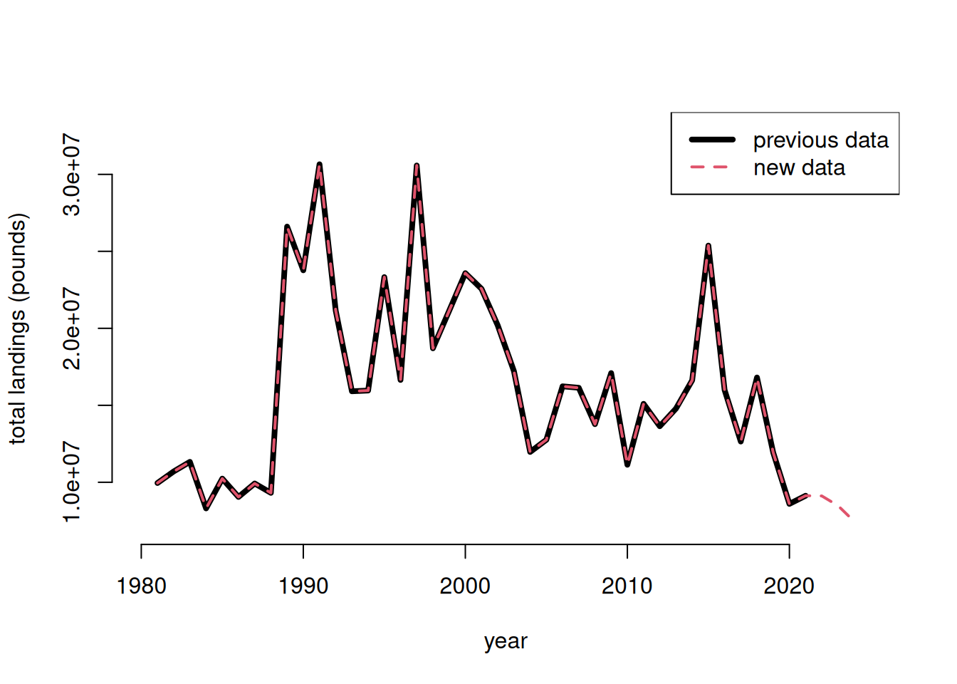
Now we can summarize the total dolphin landings in weight for the U.S. Atlantic, and compare to previous values sent for quota monitoring. We see that the values are almost identical.

# summarize by year and compare --------------------------

tot1 <- tapply(d1$LBSEST_SECWWT, d1$YEAR, sum, na.rm = T)
#head(tot1)

old <- read.csv("data/RecreationalDolphinLandings_SAandGOM_MLarkin.csv", skip = 6)
plot(old$Year, old$ATL, type = "l", xlab = "year", ylab = "total landings (pounds)", lwd = 4, 
     xlim = c(1980, 2025), ylim = c(7*10^6, 3.3*10^7), bty = "n")
lines(as.numeric(names(tot1)), tot1, lwd = 2, col = 2, lty = 2)
legend("topright", c("previous data", "new data"), col = c(1, 2), lwd = c(4, 2), lty = c(1, 2))

3.3 Partition landings by area and sector

Now we will partition out the total landings according to the dolphin MSE areas. The areas are as follows:

  • FLK: Florida Keys to Indian River County County (FL)
  • NCFL: Brevard (FL) to Southern NC (South of Hatteras)
  • NNC: Northern NC (North of Hatteras to NC/VA border)
  • VBM: Virginia to Maine
# separate out 4 regions --------------------------

d1$region <- "VBM"

# select for FLK
# FL_REG codes: 4: SE FL- Miami-Dade to Indian River County.; 5: NE FL- Brevard to Nassau County
table(d1$FL_REG, d1$NEW_STA, useNA = "always")
      
         CT   DE  FLE FLE/GA  FLW   GA   MA   MD   NC   NJ   NY   RI   SC   VA
  3       0    0    0      0  568    0    0    0    0    0    0    0    0    0
  4       0    0 1022      0    0    0    0    0    0    0    0    0    0    0
  5       0    0  312      0    0    0    0    0    0    0    0    0    0    0
  <NA>   14  114    0   1794    0   54   20  125 1344  108   73   62  644  165
      
       <NA>
  3       0
  4       0
  5       0
  <NA>    0
d1$region[which(d1$FL_REG == 3 | d1$FL_REG == 4)] <- "FLK"

# select for NCFL
d1$region[which(d1$FL_REG == 5)] <- "NCFL"
lis <- c("SC", "GA", "FLE/GA")           # NCFL states
d1$region[which(d1$NEW_STA %in% lis)] <- "NCFL"
# NC_REG codes: N: North of Cape Hatteras; S: South of Cape Hatteras
table(d1$NC_REG, d1$NEW_STA, useNA = "always")
      
         CT   DE  FLE FLE/GA  FLW   GA   MA   MD   NC   NJ   NY   RI   SC   VA
         14  114 1334   1794  568   54   20  125  586  108   73   62  644  165
  N       0    0    0      0    0    0    0    0  420    0    0    0    0    0
  S       0    0    0      0    0    0    0    0  338    0    0    0    0    0
  <NA>    0    0    0      0    0    0    0    0    0    0    0    0    0    0
      
       <NA>
          0
  N       0
  S       0
  <NA>    0
d1$region[which(d1$NC == "S")] <- "NCFL"

# select for NNC
d1$region[which(d1$NC == "N")] <- "NNC"

table(d1$FL_REG, d1$NEW_STA, d1$region)
, ,  = FLK

   
      CT   DE  FLE FLE/GA  FLW   GA   MA   MD   NC   NJ   NY   RI   SC   VA
  3    0    0    0      0  568    0    0    0    0    0    0    0    0    0
  4    0    0 1022      0    0    0    0    0    0    0    0    0    0    0
  5    0    0    0      0    0    0    0    0    0    0    0    0    0    0

, ,  = NCFL

   
      CT   DE  FLE FLE/GA  FLW   GA   MA   MD   NC   NJ   NY   RI   SC   VA
  3    0    0    0      0    0    0    0    0    0    0    0    0    0    0
  4    0    0    0      0    0    0    0    0    0    0    0    0    0    0
  5    0    0  312      0    0    0    0    0    0    0    0    0    0    0

, ,  = NNC

   
      CT   DE  FLE FLE/GA  FLW   GA   MA   MD   NC   NJ   NY   RI   SC   VA
  3    0    0    0      0    0    0    0    0    0    0    0    0    0    0
  4    0    0    0      0    0    0    0    0    0    0    0    0    0    0
  5    0    0    0      0    0    0    0    0    0    0    0    0    0    0

, ,  = VBM

   
      CT   DE  FLE FLE/GA  FLW   GA   MA   MD   NC   NJ   NY   RI   SC   VA
  3    0    0    0      0    0    0    0    0    0    0    0    0    0    0
  4    0    0    0      0    0    0    0    0    0    0    0    0    0    0
  5    0    0    0      0    0    0    0    0    0    0    0    0    0    0
table(d1$NC_REG, d1$NEW_STA, d1$region)  # check classification
, ,  = FLK

   
      CT   DE  FLE FLE/GA  FLW   GA   MA   MD   NC   NJ   NY   RI   SC   VA
       0    0 1022      0  568    0    0    0    0    0    0    0    0    0
  N    0    0    0      0    0    0    0    0    0    0    0    0    0    0
  S    0    0    0      0    0    0    0    0    0    0    0    0    0    0

, ,  = NCFL

   
      CT   DE  FLE FLE/GA  FLW   GA   MA   MD   NC   NJ   NY   RI   SC   VA
       0    0  312   1794    0   54    0    0    0    0    0    0  644    0
  N    0    0    0      0    0    0    0    0    0    0    0    0    0    0
  S    0    0    0      0    0    0    0    0  338    0    0    0    0    0

, ,  = NNC

   
      CT   DE  FLE FLE/GA  FLW   GA   MA   MD   NC   NJ   NY   RI   SC   VA
       0    0    0      0    0    0    0    0    0    0    0    0    0    0
  N    0    0    0      0    0    0    0    0  420    0    0    0    0    0
  S    0    0    0      0    0    0    0    0    0    0    0    0    0    0

, ,  = VBM

   
      CT   DE  FLE FLE/GA  FLW   GA   MA   MD   NC   NJ   NY   RI   SC   VA
      14  114    0      0    0    0   20  125  586  108   73   62    0  165
  N    0    0    0      0    0    0    0    0    0    0    0    0    0    0
  S    0    0    0      0    0    0    0    0    0    0    0    0    0    0
# summarize by Gulf and Atlantic regions and check against total -----------------------
atl <- tapply(d1$LBSEST_SECWWT, list(d1$YEAR, d1$region), sum, na.rm = T)
GULF <- tapply(dg$LBSEST_SECWWT, dg$YEAR, sum, na.rm = T)

table(rownames(atl) == names(GULF))

TRUE 
  44 
rec <- cbind(GULF, atl)

#plot(rowSums(rec), tot)
rowSums(rec)/tot
1981 1982 1983 1984 1985 1986 1987 1988 1989 1990 1991 1992 1993 1994 1995 1996 
   1    1    1   NA    1    1    1    1    1    1    1    1    1    1    1    1 
1997 1998 1999 2000 2001 2002 2003 2004 2005 2006 2007 2008 2009 2010 2011 2012 
   1    1    1    1    1    1    1    1    1    1    1    1    1    1    1    1 
2013 2014 2015 2016 2017 2018 2019 2020 2021 2022 2023 2024 
   1    1    1    1    1    1    1    1    1    1    1    1 
write.csv(rec, file = "data/recLandings.csv")

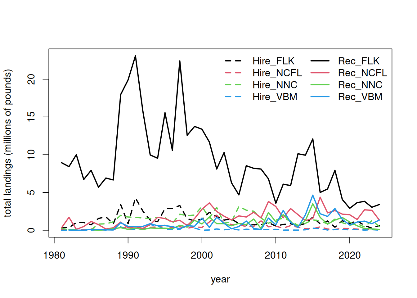
Now we will separate out the landings by recreational sector and plot the totals by region and sector.

# separate out by for hire vs. private rec --------------------------
d1$sector <- "ForHire"

d1$sector[which(d1$NEW_MODEN == "Shore")] <- "Rec"
d1$sector[which(d1$NEW_MODEN == "Priv")]  <- "Rec"

table(d1$sector, d1$NEW_MODEN, useNA = "always")    # check classification
         
           Cbt Cbt/Hbt  Hbt Priv Shore <NA>
  ForHire 1616     119 2912    0     0    0
  Rec        0       0    0 1750    22    0
  <NA>       0       0    0    0     0    0
tot <- tapply(d1$LBSEST_SECWWT, list(d1$YEAR, d1$region, d1$sector), sum, na.rm = T)

head(tot)
, , ForHire

           FLK      NCFL       NNC       VBM
1981  354639.5  74702.50 256755.24  1400.247
1982  347458.2  92271.42  27578.44  2749.224
1983 1020005.8  41784.04  88690.53  5379.177
1984 1021086.8  74658.81        NA  4203.048
1985  717523.0 172989.65  58514.13  8880.857
1986 1562354.0  63555.89 817192.26 61658.193

, , Rec

          FLK      NCFL       NNC        VBM
1981  8942641  322505.7        NA         NA
1982  8422673 1711834.7 78367.161  18727.290
1983 10000662  119370.4 44226.032   5456.237
1984  6717044  486079.7        NA      0.000
1985  7925301 1162708.4 77477.096 112944.274
1986  5699311  736872.0  2549.586 103945.134
fin <- data.frame(cbind(tot[, , 1], tot[, , 2]))
names(fin) <- c("Hire_FLK", "Hire_NCFL", "Hire_NNC", "Hire_VBM", 
                "Rec_FLK", "Rec_NCFL", "Rec_NNC", "Rec_VBM")
head(fin)
      Hire_FLK Hire_NCFL  Hire_NNC  Hire_VBM  Rec_FLK  Rec_NCFL   Rec_NNC
1981  354639.5  74702.50 256755.24  1400.247  8942641  322505.7        NA
1982  347458.2  92271.42  27578.44  2749.224  8422673 1711834.7 78367.161
1983 1020005.8  41784.04  88690.53  5379.177 10000662  119370.4 44226.032
1984 1021086.8  74658.81        NA  4203.048  6717044  486079.7        NA
1985  717523.0 172989.65  58514.13  8880.857  7925301 1162708.4 77477.096
1986 1562354.0  63555.89 817192.26 61658.193  5699311  736872.0  2549.586
        Rec_VBM
1981         NA
1982  18727.290
1983   5456.237
1984      0.000
1985 112944.274
1986 103945.134
matplot(rownames(fin), fin/10^6, lty = c(rep(2, 4), rep(1, 4)), 
        col = rep(1:4, 2), type = "l", lwd = 2, 
        xlab = "year", ylab = "total landings (millions of pounds)")
legend("topright", colnames(fin), lty = c(rep(2, 4), rep(1, 4)), col = rep(1:4, 2), lwd = 2, ncol = 2, bty = "n")

# check that totals match
cor(rowSums(fin, na.rm = T), tot1)
[1] 1
mean(rowSums(fin, na.rm = T) - tot1)   # very tiny differences
[1] 4.233284e-11

Here are the landings (in pounds) for years 1981 to 2024.

3.4 Looking at extent of discarding

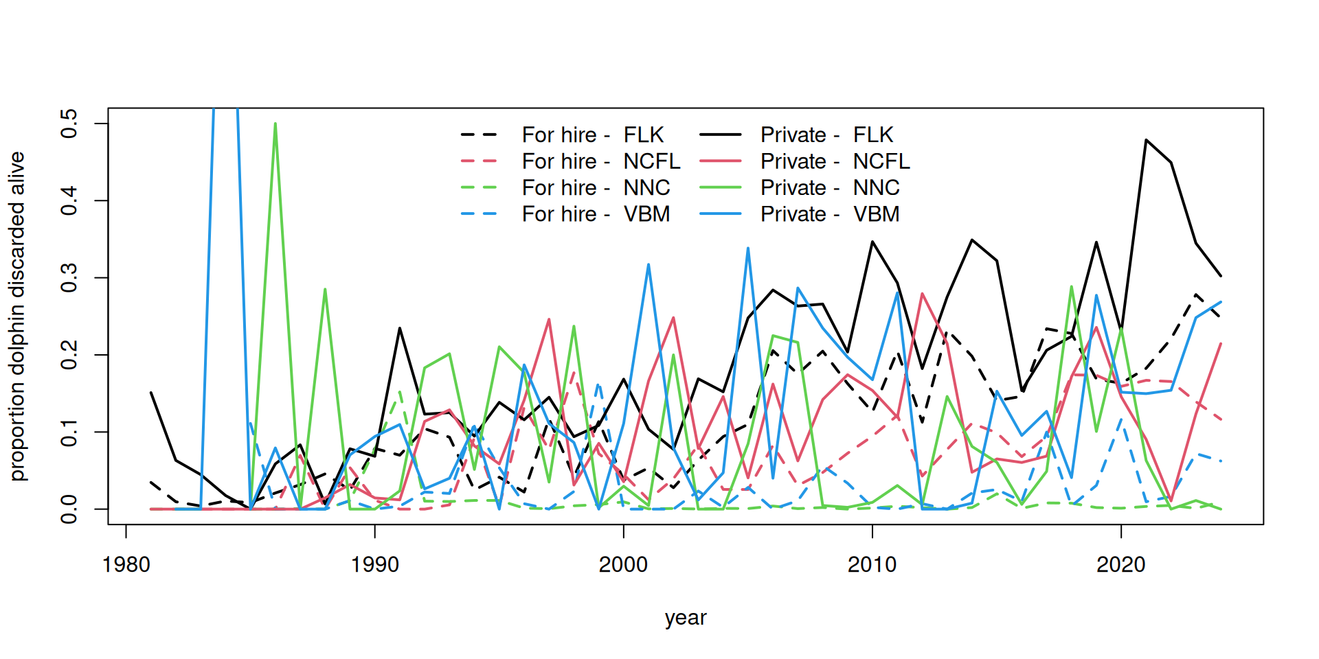
Discard estimates (known as B2 estimates) are provided in numbers by the MRIP survey but are not available in the Southeast Region Headboat Survey. We can look at the overall numbers of dolphinfish caught versus reported released from the MRIP survey to get an understanding of the extent of discarding.

d1$perdis <- d1$B2 / (d1$AB1 + d1$B2)  # percent discarded is B2 (fish released alive) / total

# calculate mean discard rate by year, region, sector ----------------
dis <- tapply(d1$perdis, list(d1$YEAR, d1$region, d1$sector), mean, na.rm = T)
disr <- tapply(d1$perdis, list(d1$region, d1$sector), mean, na.rm = T)

matplot(rownames(dis), cbind(dis[, , 1], dis[, , 2]), lty = c(rep(2, 4), rep(1, 4)), col = rep(1:4, 2), 
        type = "l", lwd = 2, xlab = "year", ylab = "proportion dolphin discarded alive", ylim = c(0, 0.5))
legend("top", c(paste("For hire - ", colnames(dis)), paste("Private - ", colnames(dis))), 
       lty = c(rep(2, 4), rep(1, 4)), col = rep(1:4, 2), lwd = 2, ncol = 2, bty = "n")

round(disr * 100, 2)  # discarding rates by region and sector
     ForHire   Rec
FLK    10.79 18.76
NCFL    9.44 11.23
NNC     0.94  9.62
VBM     2.94 12.69

According to the MRIP survey and the reported numbers, discarding generally increases over time, excluding some highly anomalous estimates from the early years which are driven by low sample sizes. Discarding is generally higher in the private sector compared to the for-hire sector, and is highest in the Florida Keys region.

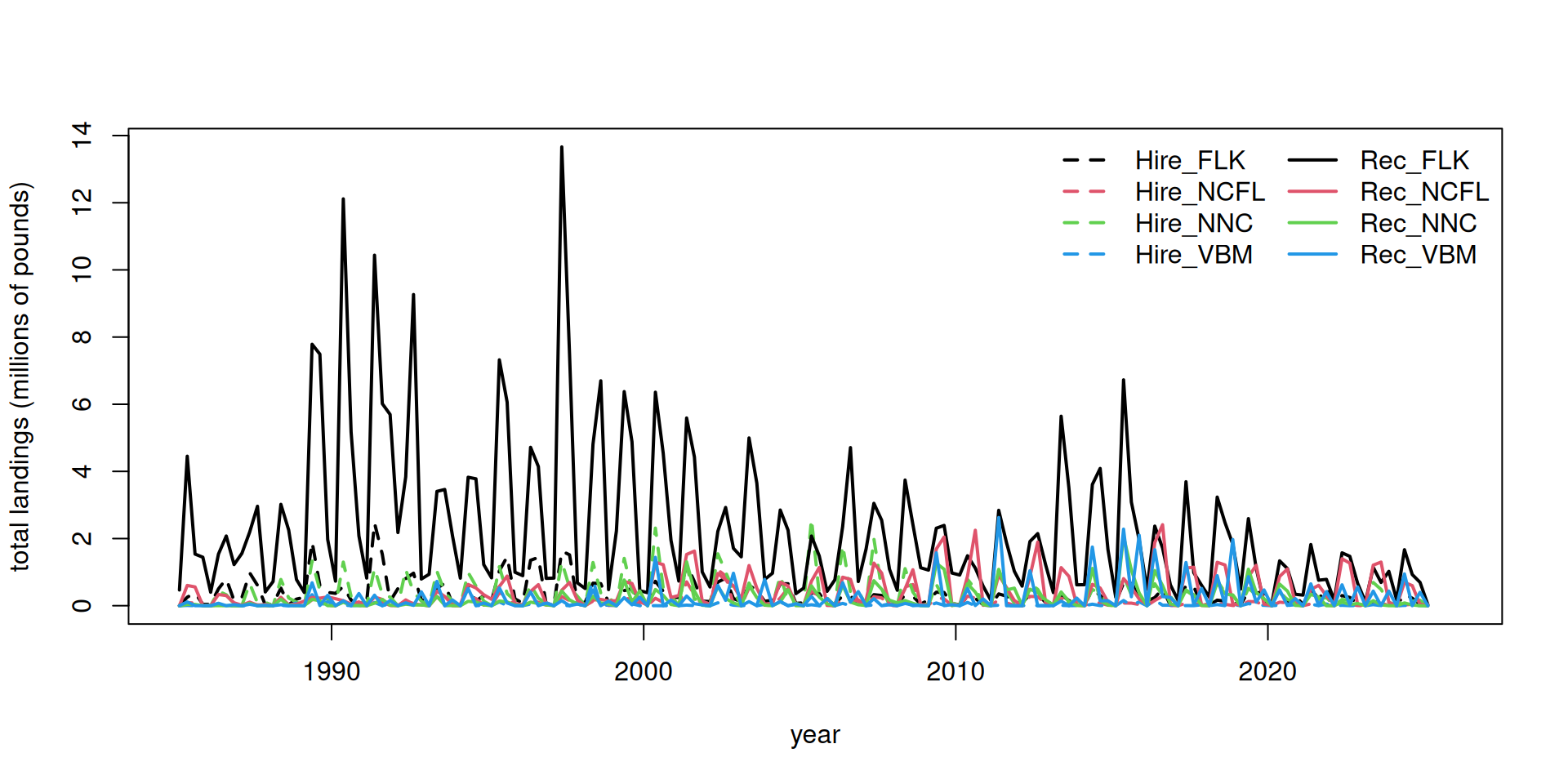
3.5 Split the landings by season

The dolphin MSE operates on a seasonal time step and thus the landings and discards must by parsed apart by individual season and year. This is not straightforward because MRIP estimates are reported in two-month waves (Jan - Feb, Mar - Apr, May - Jun, etc.), and the seasons are 3-month periods (Dec - Feb, Mar - May, Jun - Aug, Sep - Nov). For the two waves that have to be split into seasons (e.g., December is lumped with January and February; June is lumped with July and August), we split the wave 50/50%, i.e, we make the assumption that half of the landings in that wave occurs in one season and the other half occurs in the next season.

# define seasons -----------------------------
table(d1$WAVE, useNA = "always")

   0    1    2    3    4    5    6 <NA> 
   5  407  718 1230 1439 1095  581  944 
d1$YRWAVE <- paste0(d1$YEAR, "_", d1$WAVE)

totw <- tapply(d1$LBSEST_SECWWT, list(d1$YRWAVE, d1$region, d1$sector), sum, na.rm = T)

f <- data.frame(cbind(totw[, , 1], totw[, , 2]))
names(f) <- c("Hire_FLK", "Hire_NCFL", "Hire_NNC", "Hire_VBM", "Rec_FLK", "Rec_NCFL", "Rec_NNC", "Rec_VBM")
head(f)
          Hire_FLK Hire_NCFL   Hire_NNC Hire_VBM   Rec_FLK  Rec_NCFL Rec_NNC
1981_2          NA        NA         NA       NA 2793285.5 270968.46      NA
1981_3  300873.764        NA 254049.420       NA 3915698.3        NA      NA
1981_4   50017.460        NA   2705.821       NA  905621.2  51537.26      NA
1981_5    3748.301        NA         NA       NA  479834.0        NA      NA
1981_6          NA        NA         NA       NA  848201.5        NA      NA
1981_NA         NA   74702.5         NA 1400.247        NA        NA      NA
        Rec_VBM
1981_2       NA
1981_3       NA
1981_4       NA
1981_5       NA
1981_6       NA
1981_NA      NA
f$YEAR <- as.numeric(substr(rownames(f), 1, 4))
f$WAVE <- as.numeric(substr(rownames(f), 6, 8))
head(f)   # table with landings separated by wave and year
          Hire_FLK Hire_NCFL   Hire_NNC Hire_VBM   Rec_FLK  Rec_NCFL Rec_NNC
1981_2          NA        NA         NA       NA 2793285.5 270968.46      NA
1981_3  300873.764        NA 254049.420       NA 3915698.3        NA      NA
1981_4   50017.460        NA   2705.821       NA  905621.2  51537.26      NA
1981_5    3748.301        NA         NA       NA  479834.0        NA      NA
1981_6          NA        NA         NA       NA  848201.5        NA      NA
1981_NA         NA   74702.5         NA 1400.247        NA        NA      NA
        Rec_VBM YEAR WAVE
1981_2       NA 1981    2
1981_3       NA 1981    3
1981_4       NA 1981    4
1981_5       NA 1981    5
1981_6       NA 1981    6
1981_NA      NA 1981   NA
f[is.na(f)] <- 0

f <- f[which(f$YEAR >= 1985), ]
f <- f[which(f$YEAR <= 2024), ]

table(f$YEAR)

1985 1986 1987 1988 1989 1990 1991 1992 1993 1994 1995 1996 1997 1998 1999 2000 
   7    7    7    7    7    7    7    7    7    7    7    7    6    6    6    6 
2001 2002 2003 2004 2005 2006 2007 2008 2009 2010 2011 2012 2013 2014 2015 2016 
   6    6    6    6    6    6    6    6    6    6    6    6    7    7    7    6 
2017 2018 2019 2020 2021 2022 2023 2024 
   6    6    6    6    6    6    6    6 
table(f$WAVE)  

 0  1  2  3  4  5  6 
15 40 40 40 40 40 40 
# deal with NAs in many locations ---------------
# calculate percentages of landings by wave, for each region and fleet
avw <- tapply(d1$LBSEST_SECWWT, list(d1$WAVE, d1$region, d1$sector), sum, na.rm = T)
avw <- avw[-1, , ]
avw <- data.frame(cbind(avw[, , 1], avw[, , 2]))
names(avw) <- c("Hire_FLK", "Hire_NCFL", "Hire_NNC", "Hire_VBM", "Rec_FLK", "Rec_NCFL", "Rec_NNC", "Rec_VBM")
avwp <- apply(avw, 2, function (x) x / sum(x, na.rm = T)) 
#colSums(avwp)

# go through each column, find NAs and fill in waves by percentages
pre_colsum <- colSums(f, na.rm = T)  # column sums to check later

lis <- which(f$WAVE == 0)  # list of rows with NA wave data

for (i in 1:8) {      # loop through each column
  for(j in lis) {     # loop through list of NA waves
    if (f[j, i] > 0) {  # if there are NA wave landings, split by known proportion from other years
      miscatch <- avwp[, i] * f[j, i]   # missing landings are known proportion * NA wave landings
      f[which(f$YEAR == f$YEAR[j] & f$WAVE != 0), i] <- f[which(f$YEAR == f$YEAR[j] & f$WAVE != 0), i] + miscatch  # add in missing landings
      f[j, i] <- 0   # set to zero after landings is attributed to waves
    }
  }
}
f[lis, 1:8] # should be all zeros now
        Hire_FLK Hire_NCFL Hire_NNC Hire_VBM Rec_FLK Rec_NCFL Rec_NNC Rec_VBM
1985_NA        0         0        0        0       0        0       0       0
1986_NA        0         0        0        0       0        0       0       0
1987_NA        0         0        0        0       0        0       0       0
1988_NA        0         0        0        0       0        0       0       0
1989_NA        0         0        0        0       0        0       0       0
1990_NA        0         0        0        0       0        0       0       0
1991_NA        0         0        0        0       0        0       0       0
1992_NA        0         0        0        0       0        0       0       0
1993_NA        0         0        0        0       0        0       0       0
1994_NA        0         0        0        0       0        0       0       0
1995_NA        0         0        0        0       0        0       0       0
1996_NA        0         0        0        0       0        0       0       0
2013_0         0         0        0        0       0        0       0       0
2014_0         0         0        0        0       0        0       0       0
2015_0         0         0        0        0       0        0       0       0
pos_colsum <- colSums(f, na.rm = T) 
pre_colsum[1:8] == pos_colsum[1:8]  # check that landings were parsed correctly - column sums should be identical 
 Hire_FLK Hire_NCFL  Hire_NNC  Hire_VBM   Rec_FLK  Rec_NCFL   Rec_NNC   Rec_VBM 
     TRUE      TRUE      TRUE      TRUE      TRUE      TRUE      TRUE      TRUE 
f <- f[which(f$WAVE != 0), ]  # remove NA waves which now contain no landings

# split waves 3 and 6 50/50% to parse into seasons ------------------
lis <- which(f$WAVE == 3 | f$WAVE == 6)  # list of 3 and 6 waves for all years

for (i in lis) {          # go through list of waves
  temp <- f[i, ] / 2      # split landings in half
  temp[9] <- f$YEAR[i]    # reformat year and wave data columns
  temp[10] <- f$WAVE[i]
  temp <- rbind(temp, temp)   # create two half-waves and relabel with new wave reference number
  temp[1, 10] <- temp[1, 10] - 0.5
  temp[2, 10] <- temp[2, 10] + 0.5
  f <- rbind(f, temp)         # concatenate with main data table
  }

f <- f[-lis, ]  # remove waves that have been split in half

pos_colsum <- colSums(f, na.rm = T) 
pre_colsum[1:8] == pos_colsum[1:8]  # check that landings were parsed correctly - column sums should be identical 
 Hire_FLK Hire_NCFL  Hire_NNC  Hire_VBM   Rec_FLK  Rec_NCFL   Rec_NNC   Rec_VBM 
     TRUE      TRUE      TRUE      TRUE      TRUE      TRUE      TRUE      TRUE 
f <- f[order(f$YEAR, f$WAVE), ]  # reorder table in chronological order

f$YEAR[which(f$WAVE == 6.5)] <- f$YEAR[which(f$WAVE == 6.5)] + 1  # add year to December wave so it gets summed with following year
f$WAVE[which(f$WAVE == 6.5)] <- 0.5  # change December wave to small number so it gets summed with Jan/Feb

table(f$WAVE)

0.5   1   2 2.5 3.5   4   5 5.5 
 40  40  40  40  40  40  40  40 
f$seas <- cut(f$WAVE, breaks = c(0, 1.5, 3, 4.5, 6))
#table(f$seas)
f$seas1 <- NA
f$seas1[which(f$seas == "(0,1.5]")] <- "DJF"  # Dec Jan Feb is 0.5 and 1
f$seas1[which(f$seas == "(1.5,3]")] <- "MAM"  # Mar Apr May is 2 and 2.5
f$seas1[which(f$seas == "(3,4.5]")] <- "JJA"  # Jun Jul Aug is 3.5 and 4
f$seas1[which(f$seas == "(4.5,6]")] <- "SON"  # Sep Oct Nov is 5 and 5.5

temp <- tapply(f[, 1], list(f$seas1, f$YEAR), sum, na.rm = T)
temp1 <- matrix(temp)
for (i in 2:8) {
  temp2 <- matrix(tapply(f[, i], list(f$seas1, f$YEAR), sum, na.rm = T))
  temp1 <- cbind(temp1, temp2)
  }

findat <- data.frame(sort(rep(as.numeric(colnames(temp)), 4)), 
                     rep(rownames(temp), ncol(temp)), temp1)
names(findat) <- c("year", "season", names(f)[1:8])

colSums(f[, 1:8], na.rm = T) == colSums(findat[, 3:10], na.rm = T)  # check that total landings are equal before and after parsing
 Hire_FLK Hire_NCFL  Hire_NNC  Hire_VBM   Rec_FLK  Rec_NCFL   Rec_NNC   Rec_VBM 
     TRUE      TRUE      TRUE      TRUE      TRUE      TRUE      TRUE      TRUE 

We plot the results by region and sector, over the time series of year and season. We can clearly see the seasonality in the landings by region.

findat$yrseas <- findat$year + as.numeric(as.factor(findat$season))/4-0.125
matplot(findat$yrseas, findat[, 3:10]/10^6, lty = c(rep(2, 4), rep(1, 4)), col = rep(1:4, 2), type = "l", lwd = 2, 
        xlab = "year", ylab = "total landings (millions of pounds)")
legend("topright", colnames(findat[, 3:10]), lty = c(rep(2, 4), rep(1, 4)), col = rep(1:4, 2), lwd = 2, ncol = 2, bty = "n")

# check that totals match
cbind(colSums(findat[, 3:10], na.rm = T), colSums(fin[-c(1:5), ], na.rm = T))
               [,1]      [,2]
Hire_FLK   55604999  54887476
Hire_NCFL  16909916  16736926
Hire_NNC   57944903  57886388
Hire_VBM    5836953   5828072
Rec_FLK   371462933 363537632
Rec_NCFL   70803866  69641157
Rec_NNC    32556596  32479119
Rec_VBM    40081529  39968585
# the values should be close but slightly >1 because the last data set includes December 1985 data as part of 1986
colSums(findat[, 3:10], na.rm = T) / colSums(fin[-c(1:5), ], na.rm = T)
 Hire_FLK Hire_NCFL  Hire_NNC  Hire_VBM   Rec_FLK  Rec_NCFL   Rec_NNC   Rec_VBM 
 1.013073  1.010336  1.001011  1.001524  1.021800  1.016696  1.002385  1.002826 

Here we will format the data for input to the operating model.

tab3 <- findat

flt <- c(rep("Hire", nrow(tab3)*4), rep("Rec", nrow(tab3)*4))
  
yrmon <- as.numeric(tab3$yrseas)
yrs <- floor(yrmon)
qrt <- (yrmon - floor(yrmon)) * 4 + 0.5
area <- c(rep("FLK", nrow(tab3)), rep("NCFL", nrow(tab3)), 
          rep("NNC", nrow(tab3)), rep("VBM", nrow(tab3)))
area <- rep(area, 2)

findat1 <- data.frame(yrs, qrt, flt, area, matrix(as.matrix(tab3[,3:10])))
names(findat1) <- c("Year", "Quarter", "Fleet", "Area", "Catch_lbs")
head(findat1)
  Year Quarter Fleet Area Catch_lbs
1 1985       1  Hire  FLK   4462.09
2 1985       2  Hire  FLK 253487.38
3 1985       3  Hire  FLK 380811.37
4 1985       4  Hire  FLK  41469.99
5 1986       1  Hire  FLK  40545.41
6 1986       2  Hire  FLK 501184.61
#plot(findat1$Catch_lbs, type = "l")
#plot(findat1$Catch_lbs ~ factor(findat1$Area))
#plot(findat1$Catch_lbs ~ factor(findat1$Quarter))
#plot(findat1$Catch_lbs ~ factor(findat1$Year))

findat1 <- findat1[which(findat1$Year <= 2022), ]
findat1 <- findat1[which(findat1$Year >= 1986), ]
#apply(findat1, 2, table)

findat <- findat[which(findat$year >=1986 & findat$year <= 2022), ]
#check that the numbers are exactly the same
tapply(findat1$Catch_lbs, list(findat1$Area, findat1$Fleet), sum, na.rm = T)
         Hire       Rec
FLK  54012811 357091651
NCFL 16532764  65643193
NNC  56097190  32197622
VBM   5736592  37749487
colSums(findat[3:10], na.rm = T)
 Hire_FLK Hire_NCFL  Hire_NNC  Hire_VBM   Rec_FLK  Rec_NCFL   Rec_NNC   Rec_VBM 
 54012811  16532764  56097190   5736592 357091651  65643193  32197622  37749487 
# output final numbers in correct format
write.csv(findat1, file = "data/FINAL_files/rec_catch_TomFormat.csv", row.names = FALSE)