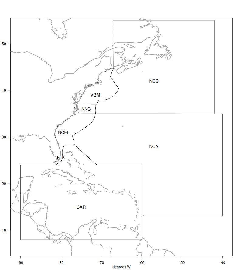
Here we define the different regions to be used in the operating model, based on the areas that were defined in the industry working groups. The operating model is intended to encompass the Western Central Atlantic dolphin population and include international waters (FAO areas 21 and 31) which are thought to be connected with the stock that is exploited by U.S. fisheries.
We use the U.S. exclusive economic zone (EEZ) to differentiate between national and international waters. Note that some U.S. commercial activity occurs in high seas waters and we will account for those catches in the summaries.
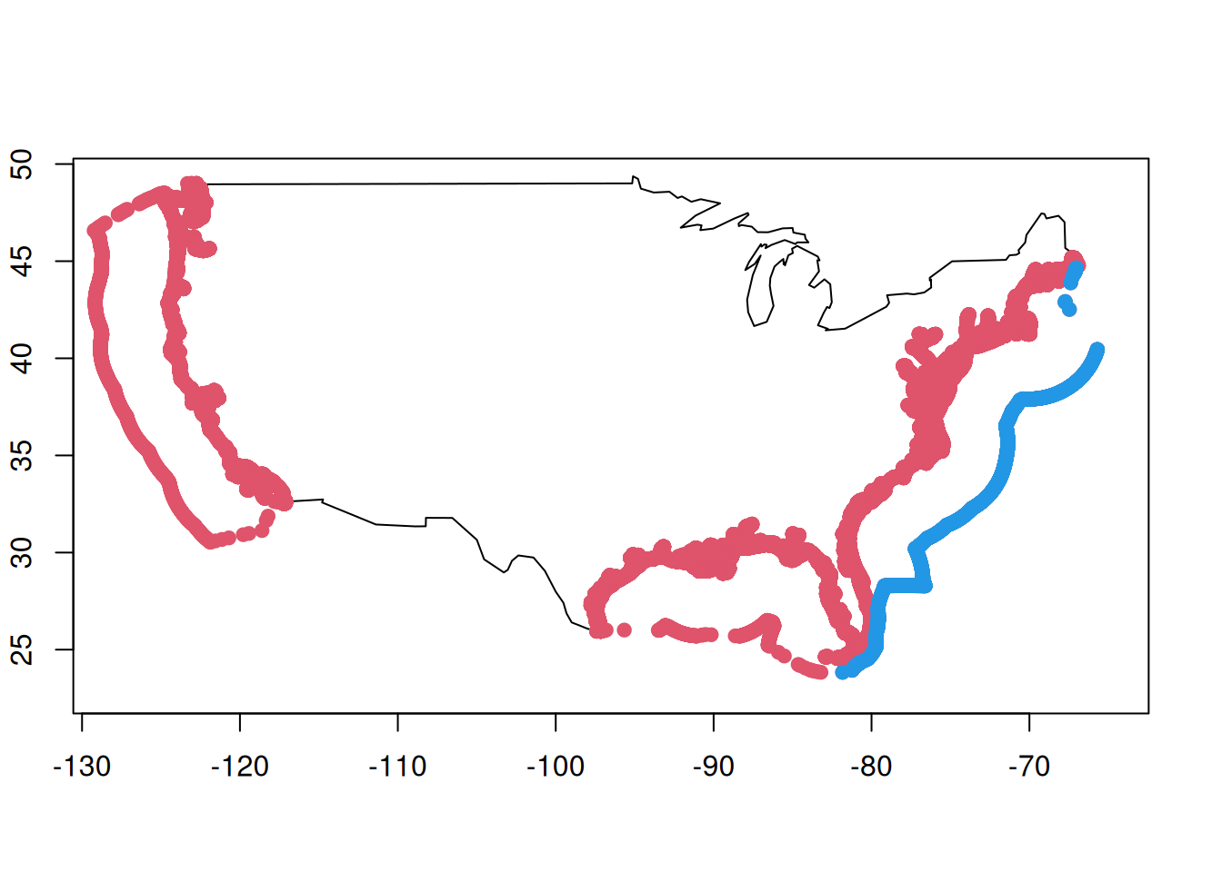
map("usa", xlim =c(-130, -63), ylim =c(22, 50))axis(1); axis(2); box()points(co$X, co$Y, pch =19, col =2)# remove points that are not in the U.S. South Atlanticco <- co[which(co$X > (-82)), ]co <- co[-which(co$X < (-81) & co$Y >25& co$Y <28), ]#plot(co$X, co$Y, col = 0)#text(co$X, co$Y, 1:nrow(co), cex = 0.7)#plot(co$X, co$Y, col = 0, xlim = c(-85, -80), ylim = c(22, 25))#text(co$X, co$Y, 1:nrow(co), cex = 0.7)# identify the northernmost and southernmost points along the Atlantic EEZco1 <- co[2100:3727, ]points(co1$X, co1$Y, col =4, pch =19)
2.2 Construct the U.S. EEZ
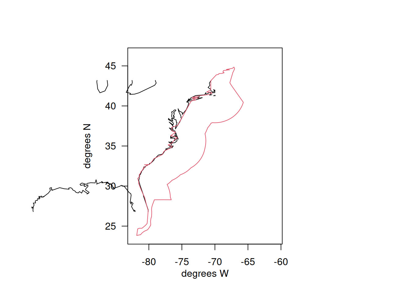
We simplify the shapefile along the U.S. coast in order to simplify computations later in the process.
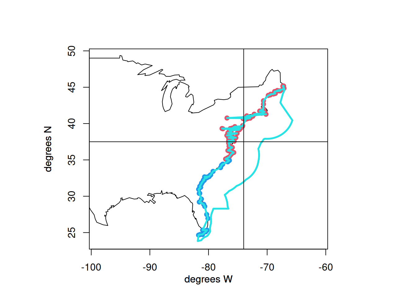
# subset points N and S of 35N for later delineationco2 <- co[-c(2100:3727), ]co3 <- co2[which(co2$Y >35), ]co4 <- co2[which(co2$Y <=35), ]# reduce number of points along the coast to make computation easierco3 <- co3[seq(1, nrow(co3), 1100), ]co4 <- co4[seq(1, nrow(co4), 800), ]map("usa", xlim =c(-100, -60), ylim =c(23, 50))mtext(side =1, "degrees W", line =2); mtext(side =2, "degrees N", line =3)mtext(side =1, "degrees W", line =2); mtext(side =2, "degrees N", line =3)axis(1); axis(2); box()points(co3$X, co3$Y, col =2, pch =19)points(co4$X, co4$Y, col =4, pch =19)co2 <-rbind(co3, co4)co2 <- co2[order(co2$Y), ]cofin <-rbind(co1, co2)polygon(cofin$X, cofin$Y, border =5, lwd =3)# make the polygon along the coast line a bit more linearabline(h =37.5)abline(v =-74)
# change the southernmost tip to exactly 24N so that it alighs with Caribbean polygoncofin <- cofin[-which(cofin$Y <24), ]cofin[1624, 2] <-24USeez <- cofin#write.csv(USeez, file = "eez.csv")
Here is a final U.S. South Atlantic EEZ polygon, with a simplified coastline to reduce computational time when subsetting data points.
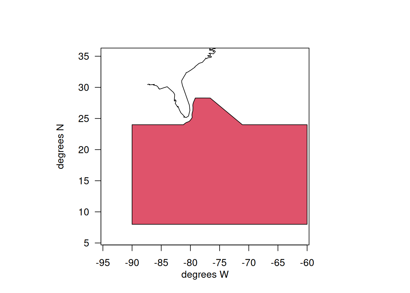
2.3 Define the Caribbean region
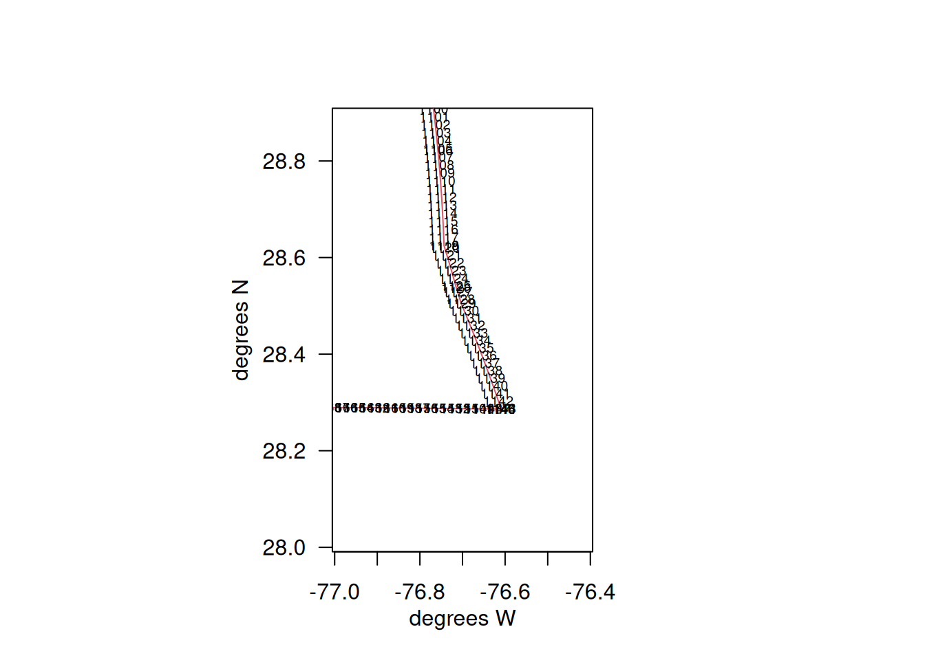
Now we define the boundaries of the Caribbean region. Its northernmost boundary aligns with the EEZ along Florida’s coast up to 28.3 degrees N, at which point the boundary cuts southeast until it intersects with the 24N boundary just east of the Bahamas, approximating the Bahamas EEZ. Its western boundary is -90 degrees W and its southern boundary is 8 degrees N (essentially the land boundary of the Caribbean Sea). Its eastern boundary is -71.1 degrees W.
which.min(cofin$Y)
[1] 1624
cofin[1624, ]
             X  Y
3723 -81.16148 24
map(database ="usa", xlim =c(-77, -76.4), ylim =c(28, 28.9))mtext(side =1, "degrees W", line =2); mtext(side =2, "degrees N", line =3)axis(1); axis(2, las =2); box()polygon(cofin$X, cofin$Y, border =2)text(cofin$X, cofin$Y, 1:nrow(cofin), cex =0.6)
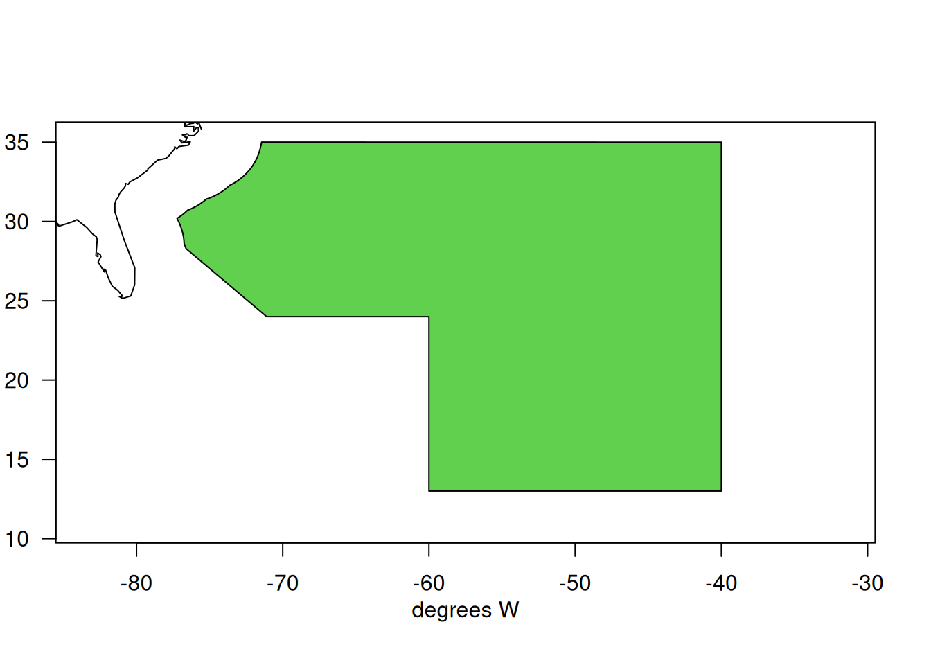
The North Central Atlantic (NCA) region, otherwise known as the Western Central Atlantic, is defined according to the boundaries of FAO area 31, but excluding the U.S. EEZ and Caribbean territorial seas to the West.
nca1 <- cofin[569:1143, ] # subset points along EEZnca2 <-data.frame(cbind(c(-71.1, -60, -60, -40, -40), c(24, 24, 13, 13, 35))) # define boundaries according to FAOnames(nca2) <-c("X", "Y")NCA <-rbind(nca1, nca2)names(NCA) <-c("X", "Y")map(database ="usa", xlim =c(-85, -30), ylim =c(10, 36)) mtext(side =1, "degrees W", line =2); mtext(side =2, "degrees N", line =3)axis(1); axis(2, las =2); box()polygon(NCA$X, NCA$Y, col =3)
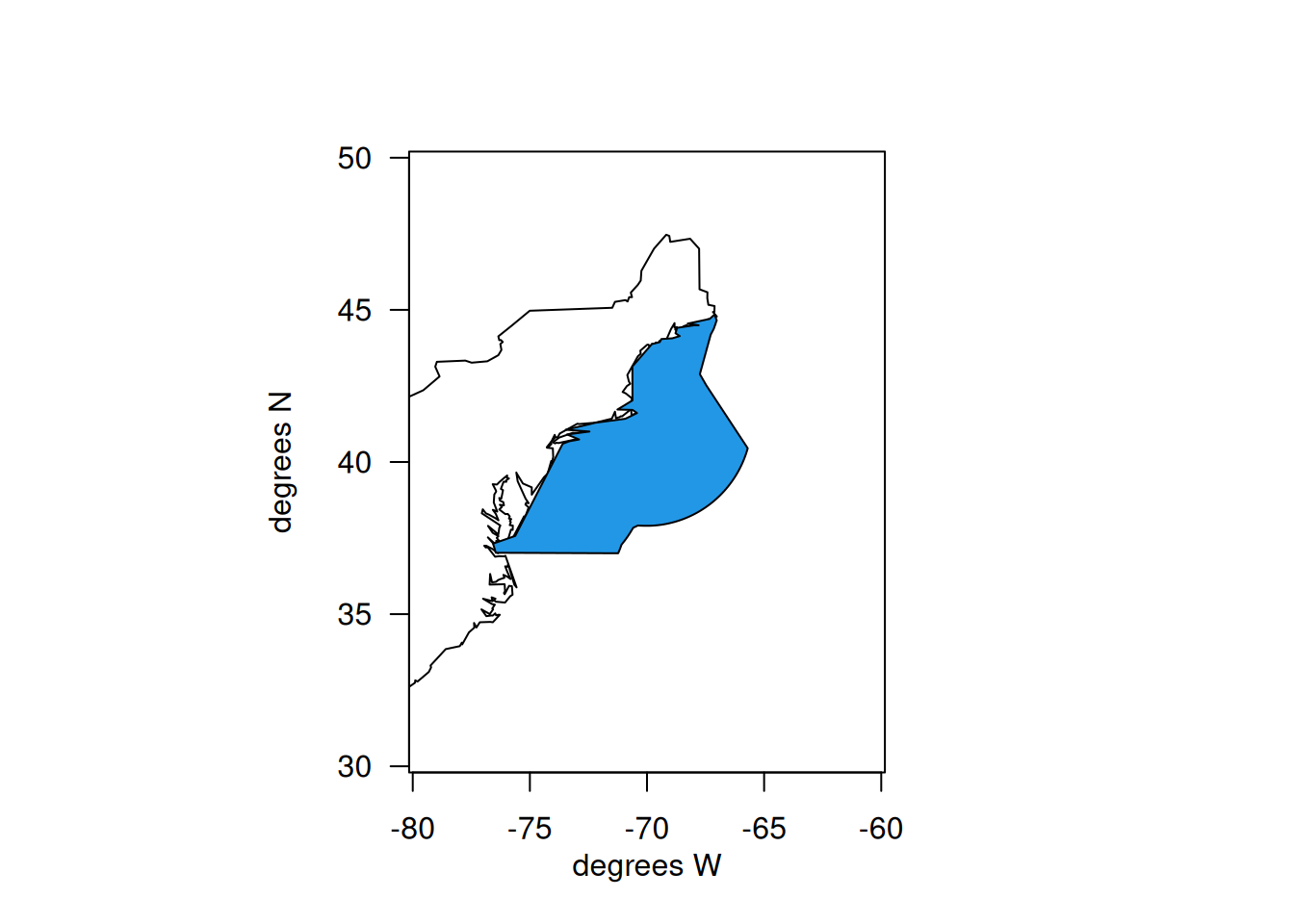
4 Define the NED region
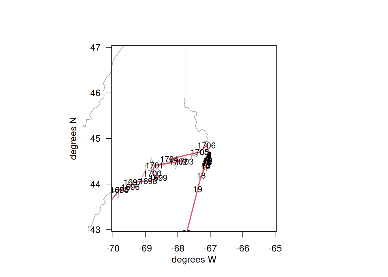
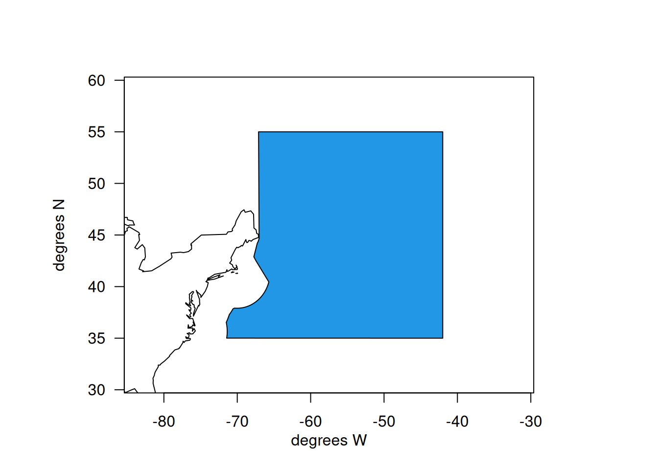
The Northeast Distant Waters (NED) region, otherwise known as the Northwesetern Atlantic, is defined according to the boundaries of FAO area 21, but excluding the U.S. EEZ territorial seas to the West. It does include Canadian and French territorial EEZs. The northern boundary is 60 degrees north, as dolphin are not caught above this latitude.
which.max(cofin$Y) # find northernmost point of U.S. EEZ
[1] 1702
cofin[1702, ]
              X        Y
77844 -67.11553 44.84764
ned1 <- cofin[1:569, ] # subset points along EEZned2 <-data.frame(cbind(c(-42, -42, -67.1), c(35, 55, 55))) # define boundaries according to FAOnames(ned2) <-c("X", "Y")NED <-rbind(ned1, ned2)names(NED) <-c("X", "Y")map(database ="usa", xlim =c(-85, -30), ylim =c(30, 60)) mtext(side =1, "degrees W", line =2); mtext(side =2, "degrees N", line =3)axis(1); axis(2, las =2); box()polygon(NED$X, NED$Y, col =4)
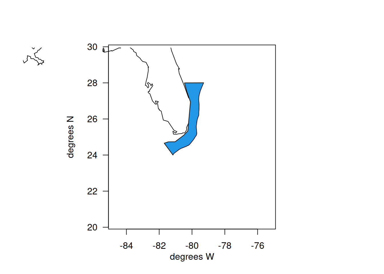
5 Define the Florida Keys region
The southernmost region of the U.S. EEZ is called the FLK region, and includes waters within the EEZ boundary, north up to 28 degrees N. The boundary of 28N is chosen because it aligns with commercial logbook reporting boundaries and aligns roughly with the Brevard - Indian River County border. This is convenient because U.S. recreational statistics are summarized as groups of counties, with SE FL encompassing Miami-Dade to Indian River County and NE FL encompassing Brevard to Nassau County.
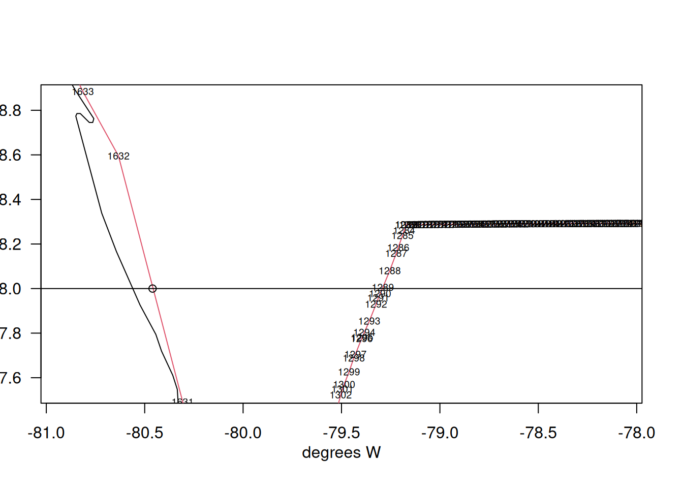
which.min(abs(co1$Y -28)) # find the southernmost point
FLK <- cofin[1289:1632, ] # subset points along EEZmap(database ="usa", xlim =c(-85, -75), ylim =c(20, 30)) mtext(side =1, "degrees W", line =2); mtext(side =2, "degrees N", line =3)axis(1); axis(2, las =2); box()polygon(FLK$X, FLK$Y, col =4)
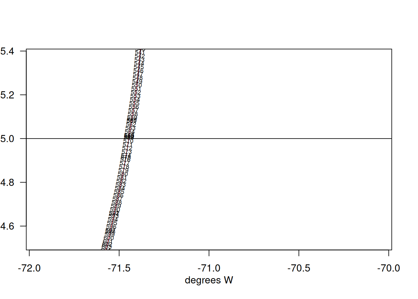
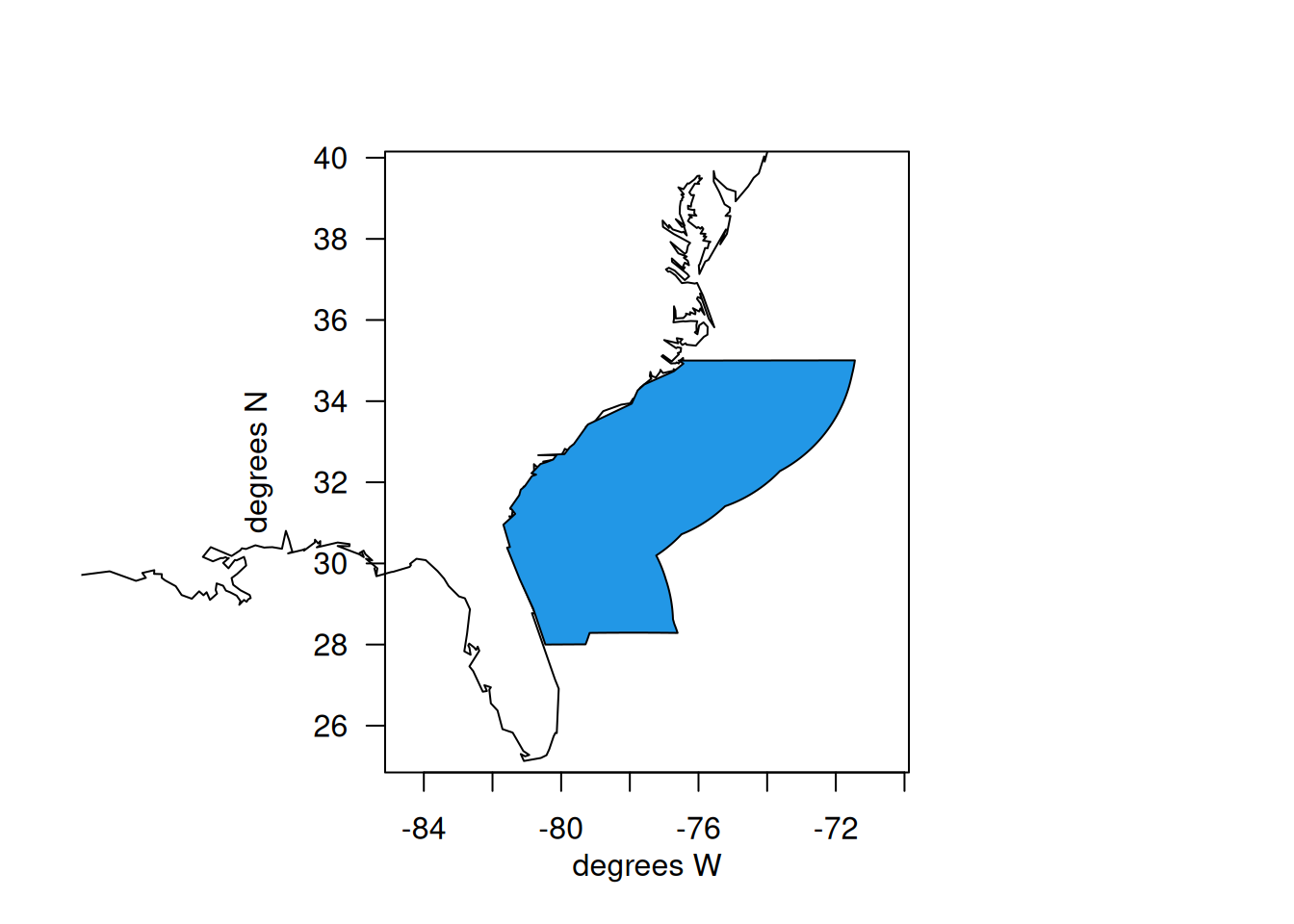
6 Define the North Florida - South NC region
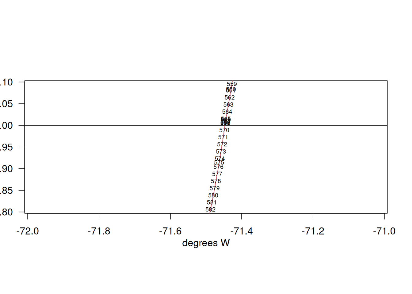
The second area that was decided upon to be defined within the operating model was northern Florida to Southern North Carolina. We form a boundary at 35 degrees north because this is the delineation between the NED and NCA regions. Also, 35N is just south of Cape Hatteras, which is a boundary for NMFS recreational data collection, as well as a boundary of commercial logbook data reporting. Therefore, all sources of data (international, U.S. commercial, and U.S. recreational) can be easily parsed along this boundary.
map(database ="usa", xlim =c(-72, -70), ylim =c(34.5, 35.4))mtext(side =1, "degrees W", line =2); mtext(side =2, "degrees N", line =3)axis(1); axis(2, las =2); box()polygon(cofin$X, cofin$Y, border =2)text(cofin$X, cofin$Y, 1:nrow(cofin), cex =0.6) # find points that fall at 35Nabline(h =35)
cofin[1663, 2] <-35NCFL <-rbind(cofin[1632:1663, ], cofin[569:1289, ]) # subset along EEZmap(database ="usa", xlim =c(-85, -70), ylim =c(25, 40)) mtext(side =1, "degrees W", line =2); mtext(side =2, "degrees N", line =3)axis(1); axis(2, las =2); box()polygon(NCFL$X, NCFL$Y, col =4)
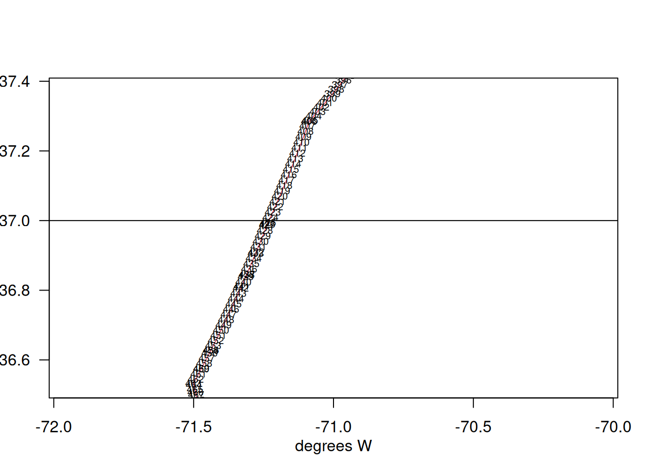
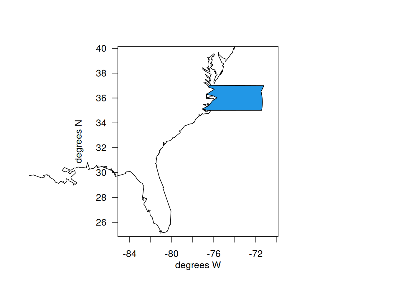
7 Define the northern North Carolina region
The third U.S. area that was decided upon to be defined within the operating model was northern North Carolina, which was intended to encompass the northern part of the state up to the Virginia border. We form a boundary at 37 degrees north because this is a boundary for commercial logbook data reporting and roughly aligns with the latitude of the state boundary between North Carolina and Virginia. Note there is a slight misalignment between this boundary and the way that U.S. recreational statistics are reported (by state), so the commercial and recreational data will be subset along slightly different boundaries for this region.