5Analysis of international catches in the high seas
Here we will explore commercial and recreational catch data as estimated by the Sea Around Us Project. This data set includes reported data for fisheries worldwide as well as reconstructed estimates for unreported catches. For each country, project scientists assemble available data on catch and use additional sociological and fishing data plus expert information and opinion, to produce their best estimates of total catch from all fishing sectors and for all species globally.
5.1 Data access and upload
The high seas data are accessed in the Basic Search High seas section of the site. The individual regions can be clicked on (e.g., Atlantic, Western Central) and then the data are downloaded using the Download Data button.
The current version of data in use is version 50.1, accessed June 2024 (the data files can be found on github in the SEFSC-dolphin-analyses/data /SAU/ folder). This was still the most recent version of data available as of September 2025.
5.2 Read in the high seas catches
First we read in the high seas catches for the Western Central Atlantic and Northwest Atlantic zones. These are equivalent to FAO areas 21 and 31.
# clear workspacerm(list =ls())if(!require("pals")) install.packages("pals")library(pals)# find data fileshslis <-dir("data/SAU/")[grep("HighSeas", dir("data/SAU/"))]# identify areas 21 and 31hslis[1]; hslis[3]
We extract the data for dolphinfish and look at the characteristics of the catches. Most of the catches are in the Western Central Atlantic, and the primary fishing entities are Venezuela and Saint Lucia. The fishing sector is all industrial, and the vast majority of the catch is reported landings, with only a tiny fraction of discards or unreported landings listed in the database. The gear type is primarily long line.
# check species name and filter out dolphinfishunique(hs$common_name)[grep("dolphin", unique(hs$common_name))]
[1] "Common dolphinfish"
hs <- hs[which(hs$common_name =="Common dolphinfish"), ]# look at the categories within each column of dataapply(hs[1:13], 2, table)
$area_name

      Atlantic, Northwest Atlantic, Western Central
                      113                       160

$area_type

high_seas
      273

$year

1985 1986 1999 2000 2001 2002 2003 2004 2005 2006 2007 2008 2009 2010 2011 2012
   1    1    1    1    1    1    1    6    4    1    5   10    5    8   10   12
2013 2014 2015 2016 2017 2018 2019
  24   22   30   33   33   29   34

$scientific_name

Coryphaena hippurus
                273

$common_name

Common dolphinfish
               273

$functional_group

Large pelagics (>=90 cm)
                     273

$commercial_group

Perch-likes
        273

$fishing_entity

                      Barbados                         Belize
                             6                              3
                        Brazil                         Canada
                            19                             18
                        Guyana                         Panama
                             1                              1
                   Saint Lucia Saint Vincent & the Grenadines
                             5                             28
                         Spain                       Suriname
                            80                              1
             Trinidad & Tobago                            USA
                            14                             74
                     Venezuela
                            23

$fishing_sector

Industrial
       273

$catch_type

Discards Landings
       5      268

$reporting_status

  Reported Unreported
       253         20

$gear_type

artisanal fishing gear           bottom trawl                gillnet
                     7                      9                     11
            hand lines               longline             mixed gear
                    17                    187                      1
         pole and line          pots or traps      unknown by source
                    19                      9                     13

$end_use_type

                         Direct human consumption    Fishmeal and fish oil
                       5                      194                       37
                   Other
                      37
# convert from metric tonnes to poundshs$pounds <- hs$tonnes *1000*2.20462# produce barplot of key data fieldspar(mar =c(3, 20, 3, 1), mfrow =c(3, 2), mex =0.5)barplot(tapply(hs$pounds/10^6, hs$area_name, sum, na.rm = T), las =2, xlab ="millions of pounds", main ="Area name", horiz = T)#barplot(tapply(hs$pounds/10^6, hs$area_type, sum, na.rm = T), las = 2, ylab = "millions of pounds", main = "Area type")#barplot(tapply(hs$pounds/10^6, hs$year, sum, na.rm = T), las = 2, ylab = "millions of pounds", main = "Year")barplot(tapply(hs$pounds/10^6, hs$fishing_entity, sum, na.rm = T), las =2, xlab ="millions of pounds", main ="Fishing entity", horiz = T)barplot(tapply(hs$pounds/10^6, hs$fishing_sector, sum, na.rm = T), las =2, xlab ="millions of pounds", main ="Fishing sector", horiz = T)barplot(tapply(hs$pounds/10^6, hs$catch_type, sum, na.rm = T), las =2, xlab ="millions of pounds", main ="Catch type", horiz = T)barplot(tapply(hs$pounds/10^6, hs$reporting_status, sum, na.rm = T), las =2, xlab ="millions of pounds", main ="Reporting status", horiz = T)barplot(tapply(hs$pounds/10^6, hs$gear_type, sum, na.rm = T), las =2, xlab ="millions of pounds", main ="Gear type", horiz = T)
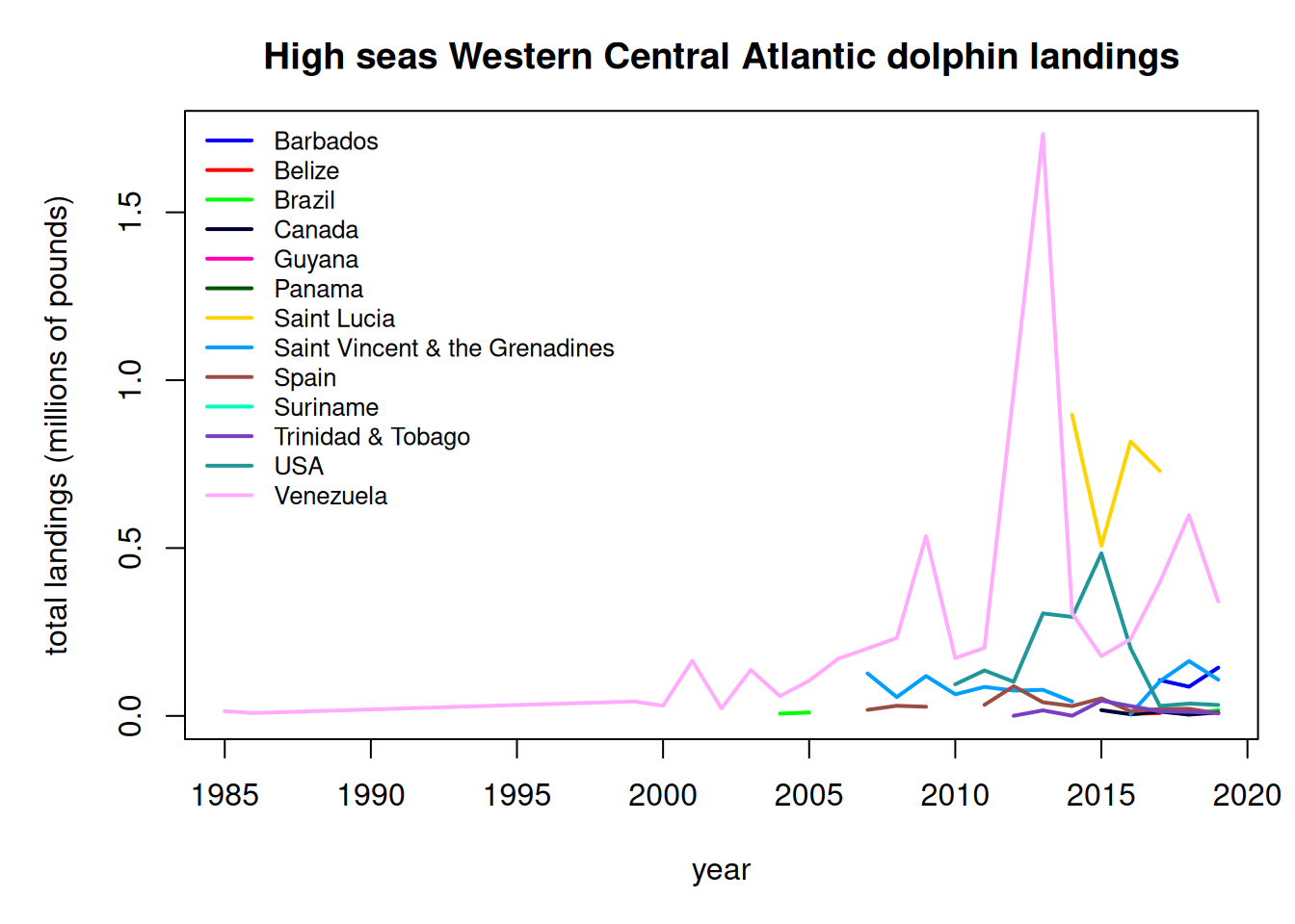
We plot the annual landings by fishing entity to look at trends over time.
hs$fishing_entity <-as.factor(hs$fishing_entity)hs$fishing_entity <-droplevels(hs$fishing_entity)par(mar =c(5, 5, 3, 1), mfrow =c(1, 1))tab <-tapply(hs$pounds, list(hs$year, hs$fishing_entity), sum, na.rm = T)matplot(as.numeric(rownames(tab)), tab/10^6, type ="l", col =glasbey(ncol(tab)), lty =1, lwd =2, xlab ="year", ylab ="total landings (millions of pounds)", main ="High seas Western Central Atlantic dolphin landings")legend("topleft", colnames(tab), col =glasbey(ncol(tab)), lty =1, lwd =2, cex =0.8, bty ="n")
Finally we output the subset of high seas dolphin landings for the two areas. Because we have already accounted for the USA landings in our national reporting and are aiming to only summarize international landings here, we filter out the USA landings from the Sea Around Us database.
# write summary to merge with EEZ data write.csv(tab, file ="data/SAU/high_seas_by_year.csv")
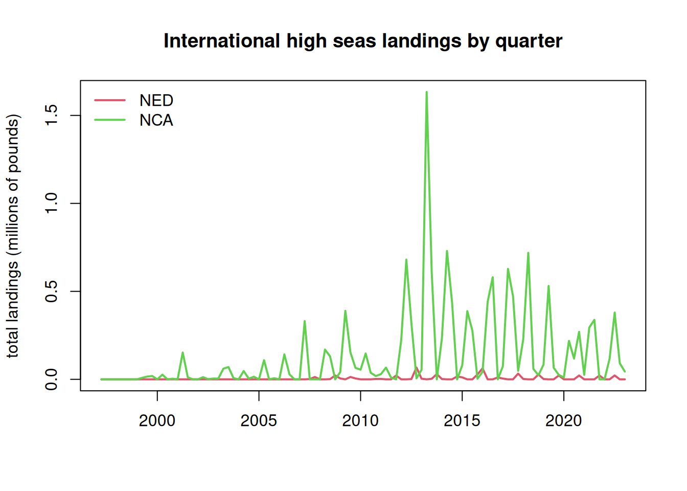
5.4 Distribute the high seas landings across quarters of the year
The international landings are only reported as annual landings and do not have any month or season associated with them. However, the MSE operating model requires seasonal landings. The majority of the international landings are caught by longline, so we will assume that the fleet distribution of the U.S. pelagic longline is representative of the seasonality of the international high seas fleets. Now we parse the annual landings according to the seasonality of the U.S. fleet.
At the time of analysis, the SAU database only contained landings to 2019, so we interpolated the 2019 values to cover years 2020 - 2022.
# read in the percentage of the landings by area and year-quarter combinations from the U.S. PLLload("data/outputs/per_PLLcatch_by_area_yearquarter.RData") tab <- tab[which(rownames(tab) >=1997), ] # PLL data are only available from 1997 on #tab[nrow(tab), ]tab <-rbind(tab, tab[nrow(tab), ], tab[nrow(tab), ], tab[nrow(tab), ]) # interpolate 2019 landings for 2020-2022tail(tab)
     Atlantic, Northwest Atlantic, Western Central
2017            34806.93                 1374259.7
2018            29328.36                  885814.8
2019            21870.62                  632747.2
                21870.62                  632747.2
                21870.62                  632747.2
                21870.62                  632747.2
NED <- percatch[, , 1] # create matrices for final landings dataNCA <- percatch[, , 1]for (i in1:ncol(percatch)) { NED[, i] <- percatch[, i, 7] * tab[i, 1] # these are the percentages for the NED (Atlantic Northwest) NCA[, i] <- percatch[, i, 1] * tab[i, 2] # these are the percentages for the NCA (Western Central Atlantic) }# plot the parsed out data by year-quarteryrs <-sort(rep(as.numeric(colnames(NCA)), 4))qrt <-rep(1:4, length(yrs)/4)matplot(yrs + qrt/4, cbind(matrix(NED), matrix(NCA))/10^6, lty =1, lwd =2, col =2:3, type ="l", main ="International high seas landings by quarter", xlab ="", ylab ="total landings (millions of pounds)")legend("topleft", c("NED", "NCA"), lwd =2, col =2:3, bty ="n")
# save NED data in this format because it needs to be combined with Canadian EEZ landingssave(NED, file ="data/outputs/NED_year_quarter.RData")
Finally, we format the data in the format for input into the operating model. We only include NCA here, as the NED high seas landings must be combined with international landings in territorial waters of Canada and France in the NED region.
# format for operating modelflt <-rep("Intl", length(yrs))are <-rep("NCA", length(yrs))findat <-data.frame(cbind(yrs, qrt, flt, are, matrix(NCA)))names(findat) <-c("Year", "Quarter", "Fleet", "Area", "Catch_lbs")findat$Catch_lbs <-as.numeric(findat$Catch_lbs)head(findat)