6Analysis of international catches in territorial waters
6.1 Data access and upload
For catches within each country’s exclusive economic zones, data are downloaded from the Sea Around Us site (Pauly, Zeller, and Palomares, 2020.). In the Biodiversity by Taxon Tools and Data, we filter by EEZ for All regions, and then filter by Taxon at the Species level for Common dolphinfish (Coryphaena hippurus). After clicking “View graphs” one can access the full data set using the “Download Data” button.
6.2 Read in the catches within excluzive economic zones (EEZs)
Now we read in the catches reported by each country or jurisdiction’s respective EEZ. Because we have extracted dolphin catches for EEZs worldwide, we need to separate out the catches for the Atlantic Ocean basin.
# load librarieslibrary(pals)rm(list =ls())d <-read.csv("data/SAU/SAU Taxa 600006 v50-1.csv", header = T, sep =",") # v. 50.1 - June 2024head(d)
     area_name area_type year     scientific_name        common_name
1    Australia       eez 1950 Coryphaena hippurus Common dolphinfish
2    Australia       eez 1950 Coryphaena hippurus Common dolphinfish
3    Australia       eez 1950 Coryphaena hippurus Common dolphinfish
4      Bahamas       eez 1950 Coryphaena hippurus Common dolphinfish
5     Barbados       eez 1950 Coryphaena hippurus Common dolphinfish
6 Bermuda (UK)       eez 1950 Coryphaena hippurus Common dolphinfish
          functional_group commercial_group fishing_entity fishing_sector
1 Large pelagics (>=90 cm)      Perch-likes      Australia     Industrial
2 Large pelagics (>=90 cm)      Perch-likes      Australia     Industrial
3 Large pelagics (>=90 cm)      Perch-likes      Australia     Industrial
4 Large pelagics (>=90 cm)      Perch-likes        Bahamas   Recreational
5 Large pelagics (>=90 cm)      Perch-likes       Barbados   Recreational
6 Large pelagics (>=90 cm)      Perch-likes   Bermuda (UK)      Artisanal
  catch_type reporting_status                 gear_type
1   Landings         Reported                  longline
2   Landings         Reported                  longline
3   Landings         Reported                  longline
4   Landings       Unreported recreational fishing gear
5   Landings       Unreported recreational fishing gear
6   Landings         Reported         small scale lines
              end_use_type       tonnes landed_value
1    Fishmeal and fish oil  0.003373202 3.438170e-05
2 Direct human consumption  6.739657104 1.040254e+04
3                    Other  0.003373202 3.438170e-05
4 Direct human consumption 48.665105143 8.262728e+00
5 Direct human consumption  0.009158559 4.846886e-04
6 Direct human consumption  1.511085514 3.199403e+03
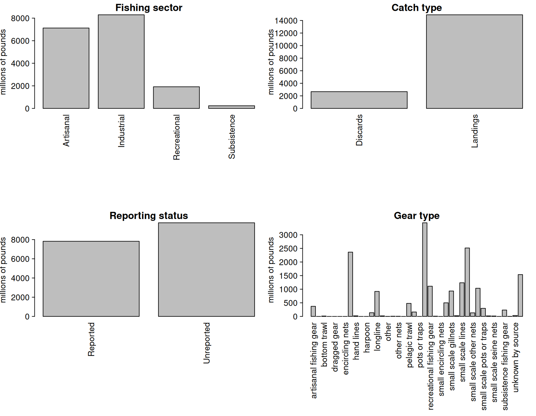
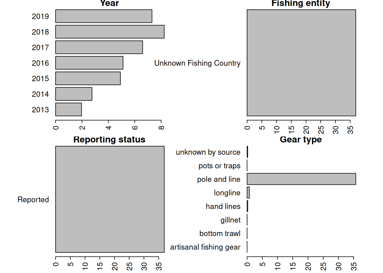
We look at the characteristics of the catches within EEZs. These are largely industrial and artisanal in nature. Landings are the majority of the catch but discards are also present. There are more unreported landings than reported landings and a variety of gear types are used.
# look at characteristics of data par(mfrow =c(2, 2), mar =c(20, 7, 3, 1), mex =0.5, mgp =c(5.5, 1, 0))barplot(tapply(d$lbs, d$fishing_sector, sum, na.rm = T)/10^6, las =2, ylab ="millions of pounds", main ="Fishing sector")barplot(tapply(d$lbs, d$catch_type, sum, na.rm = T)/10^6, las =2, ylab ="millions of pounds", main ="Catch type")barplot(tapply(d$lbs, d$reporting_status, sum, na.rm = T)/10^6, las =2, ylab ="millions of pounds", main ="Reporting status")barplot(tapply(d$lbs, d$gear_type, sum, na.rm = T)/10^6, las =2, ylab ="millions of pounds", main ="Gear type")
Now we have to manually assign the different EEZs to respective areas. We separate the geographical areas within the Atlantic Ocean (North and South) and lump all other EEZs into “other oceans.” This latter category is largely the Pacific Ocean and to a lesser extent the Indian Ocean. We remove the high seas catch from this database as it is not ocean-specific and we have extracted the ocean-specific high seas catch previously.
# remove the high seas catch from this databased <- d[which(d$area_type !="high_seas"), ] d$fishing_entity <-as.factor(d$fishing_entity)d$fishing_entity <-droplevels(d$fishing_entity)table(d$area_type) # this should be all "eez"
  eez
63056
# Western Central Atlantic EEZsWCA <-c("Bahamas", "Barbados", "Cayman Isl. (UK)", "Dominica", "Dominican Republic", "Grenada", "Aruba (Netherlands)", "Haiti", "Guadeloupe (France)", "Jamaica", "Martinique (France)","Montserrat (UK)", "Nicaragua (Caribbean)", "Puerto Rico (USA)", "Saint Kitts & Nevis", "Saint Lucia", "Saint Vincent & the Grenadines", "Trinidad & Tobago", "US Virgin Isl.", "St Barthelemy (France)", "St Martin (France)", "Curaçao (Netherlands)", "Bonaire (Netherlands)","Saba and Sint Eustatius (Netherlands)", "Sint Maarten (Netherlands)", "Honduras (Caribbean)","Colombia (Caribbean)", "Mexico (Atlantic)", "Turks & Caicos Isl. (UK)", "Guyana", "Venezuela","Antigua & Barbuda", "Belize", "British Virgin Isl. (UK)", "French Guiana", "Cuba", "Anguilla (UK)", "Suriname", "Costa Rica (Caribbean)", "Guatemala (Caribbean)", "Panama (Caribbean)", "Bermuda (UK)", "Curaçao (Netherlands)") # BrazilBra <-c("Brazil (mainland)", "Fernando de Noronha (Brazil)", "St Paul and St. Peter Archipelago (Brazil)")# CanadaCan <-c("Canada (East Coast)", "Saint Pierre & Miquelon (France)")# United StatesUSA <-c("USA (East Coast)", "USA (Gulf of Mexico)")# Northeast Atlantic EEZsNEA <-c("Canary Isl. (Spain)", "Spain (mainland; Med and Gulf of Cadiz)", "Spain (Northwest)", "Spain (mainland, Med and Gulf of Cadiz)", "France (Atlantic Coast)", "Portugal (mainland)", "Azores Isl. (Portugal)")# Eastern Central Atlantic EEZsECA <-c("Madeira Isl. (Portugal)", "Cape Verde", "Equatorial Guinea", "Benin", "Sao Tome & Principe ", "Sao Tome & Principe", "Morocco (Central)", "Ghana", "Côte d'Ivoire", "Côte d'Ivoire", "Guinea", "Liberia", "Sierra Leone", "Nigeria", "Togo", "Guinea-Bissau", "Senegal", "Cameroon", "Gambia", "Mauritania", "Morocco (South)", "Gabon", "Congo; R. of", "Congo, R. of", "Congo (ex-Zaire)")# Southeastern Atlantic EEZsSEA <-c("Angola", "Namibia", "South Africa (Atlantic and Cape)", "Ascension Isl. (UK)", "Saint Helena (UK)", "Tristan da Cunha Isl. (UK)")# Southwest Atlantic EEZsSWA <-c("Trindade & Martim Vaz Isl. (Brazil)", "Uruguay")# Mediterranean EEZsMed <-c("Italy (mainland)", "Libya", "Malta", "Syria", "Sicily (Italy)","Sardinia (Italy)", "Balearic Islands (Spain)", "Cyprus (North)", "Cyprus (South)", "Gaza Strip", "Greece (without Crete)", "Crete (Greece)", "Lebanon", "Turkey (Mediterranean Sea)", "Egypt (Mediterranean)", "Israel (Mediterranean)", "Tunisia", "Algeria", "Albania", "Croatia", "Montenegro", "Morocco (Mediterranean)", "France (Mediterranean)", "Corsica (France)")# add variable to specify regiond$reg <-"other oceans"d$reg[which(d$area_name %in% WCA)] <-"Western Central Atlantic EEZs"d$reg[which(d$area_name %in% Bra)] <-"Brazil EEZ"d$reg[which(d$area_name %in% Can)] <-"Canadian EEZ"d$reg[which(d$area_name %in% USA)] <-"United States EEZ"d$reg[which(d$area_name %in% NEA)] <-"Northeast Atlantic EEZs"d$reg[which(d$area_name %in% ECA)] <-"Eastern Central Atlantic EEZs"d$reg[which(d$area_name %in% SEA)] <-"Southeast Atlantic EEZs"d$reg[which(d$area_name %in% SWA)] <-"Southwest Atlantic EEZs"d$reg[which(d$area_name %in% Med)] <-"Mediterranean Sea EEZs"
Now we will check that we have classified the regions correctly.
# check region designation othlis <-unique(d$area_name[which(d$reg =="other oceans")])print("EEZs of all other oceans: ")
Now we summarize the catch by region by grouping the catch across the EEZs by region. We save these data for later analysis, and move on to analyzing only the Western Central and Northwest Atlantic jurisdictions.
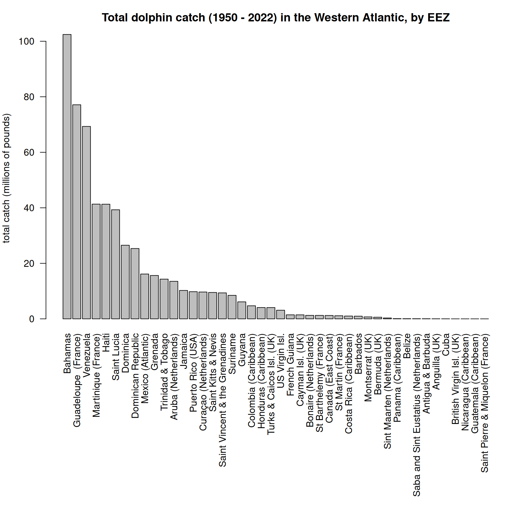
# summarize EEZ catch by regiontab <-tapply(d$lbs, list(d$year, d$reg), sum, na.rm = T)write.csv(data.frame(tab), file ="data/outputs/intl_catches_allAtlantic.csv", row.names = T)dwest <- d[which(d$reg =="Canadian EEZ"| d$reg =="Western Central Atlantic EEZs"), ]save(dwest, file ="data/outputs/SAU_EEZs_WCA.RData")tab <-tapply(dwest$lbs, list(dwest$year, dwest$area_name), sum, na.rm = T)# eight countries are responsible for vast majority of catch with total catches across all years exceeding 20M poundspar(mar =c(17, 4, 3, 1))barplot(sort(colSums(tab, na.rm = T)/10^6, decreasing = T), horiz = F, las =2,main ="Total dolphin catch (1950 - 2022) in the Western Atlantic, by EEZ", ylab ="total catch (millions of pounds)")
Note that Bermuda is actually in the NCA region and not the Greater Caribbean region. However, its catches constitute 0.1% of the total catch which is essentially negligible, and to avoid complicating the operating model and code unnecessarily we will leave those catches accounted for in the CAR region.
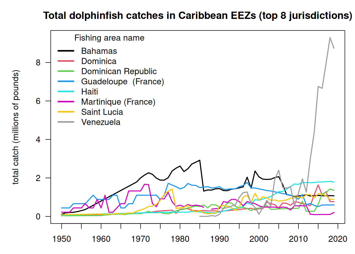
lis <-names(sort(colSums(tab, na.rm = T), decreasing = T)[1:8]) # list of top 8 jurisdictionstab1 <- tab[, colnames(tab) %in% lis]par(mar =c(3, 5, 3, 1))matplot(rownames(tab1), tab1/10^6, las =2, type ="l", lty =1, lwd =2, pch =19, col =1:8,xlab ="", ylab ="total catch (millions of pounds)", axes = F, main ="Total dolphinfish catches in Caribbean EEZs (top 8 jurisdictions)")axis(1, at =seq(1950, 2020, 5)); axis(2, las =2); box()legend("topleft", colnames(tab1), col =1:8, lty =1, lwd =3, bty ="n", title ="Fishing area name")
Note the rapid eight-fold increase in catches listed within the Venezuelan EEZ which occurs from 2013 - 2019. This increase is responsible for a rapid increase in estimated international catches within the Western Atlantic.
6.5 Look at Venezuela catches in detail
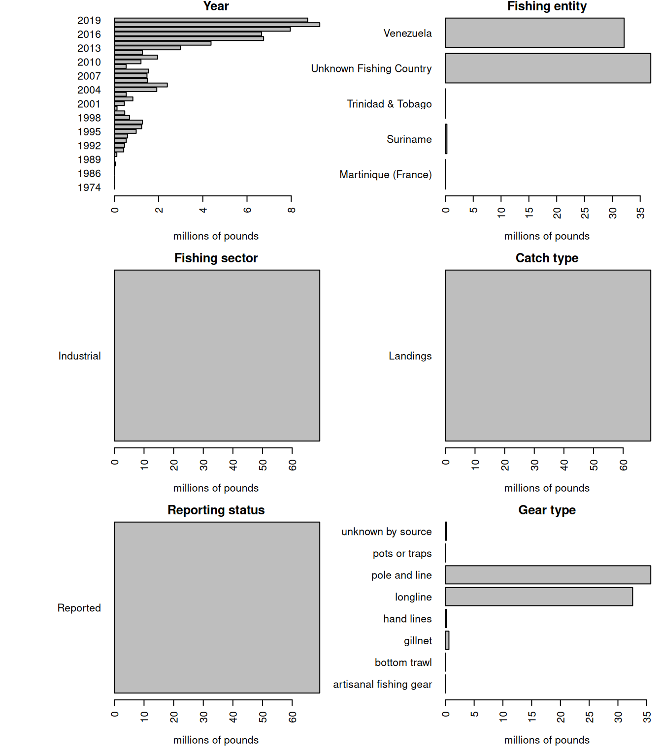
The figures above indicate that the database shows a rapid increase in international catches within the Western Atlantic, driven by a sudden increase in catches reported within Sea Around Us database within the Venezuelan EEZ. We investigate these catches in detail, as it seems odd that a relatively small fleet from a single country would be able to ramp up effort so rapidly. Data can be downloaded on a country-specific basis, the catches by taxon in the waters of Venezuela are accessed here.
rm(list =ls()) # clear the workspace# download the data for waters of Venezuelaven <-read.csv("data/SAU/SAU EEZ 862 v50-1.csv") # subset dolphinfish from the datav <- ven[which(ven$common_name =="Common dolphinfish"), ]#apply(v[1:13], 2, table)#convert to poundsv$pounds <- v$tonnes *1000*2.20462# look at the characteristics of the datapar(mar =c(5, 10, 1, 1), mfrow =c(3, 2), mex =0.9)#barplot(tapply(v$pounds/10^6, v$area_name, sum, na.rm = T), las = 2, xlab = "millions of pounds", main = "Area name", horiz = T)#barplot(tapply(v$pounds/10^6, v$area_type, sum, na.rm = T), las = 2, xlab = "millions of pounds", main = "Area type", horiz = T)barplot(tapply(v$pounds/10^6, v$year, sum, na.rm = T), las =2, xlab ="millions of pounds", main ="Year", horiz = T)barplot(tapply(v$pounds/10^6, v$fishing_entity, sum, na.rm = T), las =2, xlab ="millions of pounds", main ="Fishing entity", horiz = T)barplot(tapply(v$pounds/10^6, v$fishing_sector, sum, na.rm = T), las =2, xlab ="millions of pounds", main ="Fishing sector", horiz = T)barplot(tapply(v$pounds/10^6, v$catch_type, sum, na.rm = T), las =2, xlab ="millions of pounds", main ="Catch type", horiz = T)barplot(tapply(v$pounds/10^6, v$reporting_status, sum, na.rm = T), las =2, xlab ="millions of pounds", main ="Reporting status", horiz = T)barplot(tapply(v$pounds/10^6, v$gear_type, sum, na.rm = T), las =2, xlab ="millions of pounds", main ="Gear type", horiz = T)
Note that a large portion of the catch in the database is listed as coming from an “Unknown Fishing Country.” We extract these catches and further investigate the characteristics.
# extract the Unknown Fishing Country catchv1 <- v[which(v$fishing_entity =="Unknown Fishing Country"), ]#apply(v1[1:15], 2, table)# look at characteristicspar(mar =c(3, 10, 1, 5), mfrow =c(2, 2), mex =0.6)barplot(tapply(v1$pounds/10^6, v1$year, sum, na.rm = T), las =2, xlab ="millions of pounds", main ="Year", horiz = T)barplot(tapply(v1$pounds/10^6, v1$fishing_entity, sum, na.rm = T), las =2, xlab ="millions of pounds", main ="Fishing entity", horiz = T)barplot(tapply(v1$pounds/10^6, v1$reporting_status, sum, na.rm = T), las =2, xlab ="millions of pounds", main ="Reporting status", horiz = T)barplot(tapply(v1$pounds/10^6, v1$gear_type, sum, na.rm = T), las =2, xlab ="millions of pounds", main ="Gear type", horiz = T)
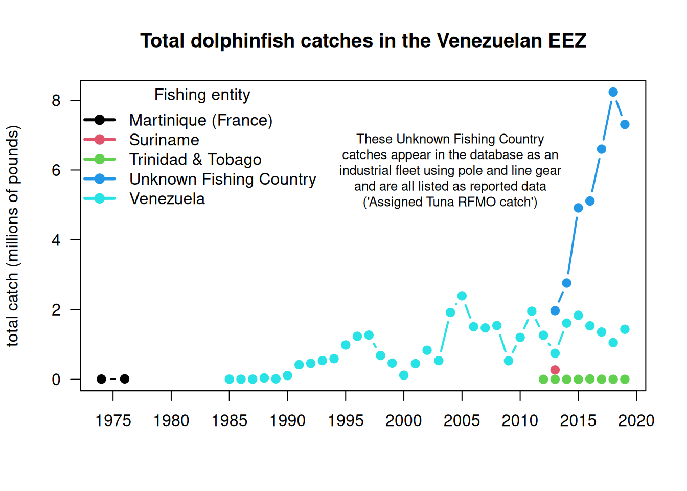
Here is another look at the catches within the venezuelan EEZ, separated by fishing entity.
     Martinique (France) Suriname Trinidad & Tobago Unknown Fishing Country
1974            7320.429       NA                NA                      NA
1976           12814.641       NA                NA                      NA
1985                  NA       NA                NA                      NA
1986                  NA       NA                NA                      NA
1987                  NA       NA                NA                      NA
1988                  NA       NA                NA                      NA
     Venezuela
1974        NA
1976        NA
1985  4699.563
1986  2229.484
1987  4585.610
1988 39960.149
matplot(rownames(tab), tab/10^6, las =2, type ="b", lty =1, lwd =2, pch =19, col =1:5,xlab ="", ylab ="total catch (millions of pounds)", axes = F, main ="Total dolphinfish catches in the Venezuelan EEZ")axis(1, at =seq(1950, 2020, 5)); axis(2, las =2); box()legend("topleft", colnames(tab), col =1:5, pch =19, lty =1, lwd =3, bty ="n", title ="Fishing entity")text(2004, 6, cex =0.8,"These Unknown Fishing Country\ncatches appear in the database as an\nindustrial fleet using pole and line gear\nand are all listed as reported data\n('Assigned Tuna RFMO catch')")
The very substantial increase in international Western Atlantic dolphin catches can be attributed solely to this Unknown Fishing Country catches which appear in the database beginning in 2013. The documentation of the catch reconstruction can be found in the Sea Around Us documentation files (see Mendoza et al. 2015). We spoke to Jeremy Mendoza and other experts who were involved in the reconstruction of domestic catches in Venezuela, and they noted that the “Assigned tuna RFMO catch” actually emerge from spatially reshuffled landing reports to ICCAT, according to the methods of Coulter et al. (2020). In this work, the Sea Around Us team developed a global spatial reallocation of landings of tunas and associated species that were reported to ICCAT. In short, this work uses the fraction of reported spatially disaggregated data to reallocate all data reported to ICCAT. This step is necessary because there are not many countries that report spatial data to ICCAT in the region, and this method may lead to a significant reallocation of landings from the Caribbean to the Venezuelan EEZ, where the local pole and line fishery is significant (J. Mendoza, personal communication). Thus, it is likely that landings from other EEZs, that were included in the reconstructed catch data layer, could have been reassigned to the Venezuelan EEZ.
Because there may be some overlap between the reconstructed data used in the national EEZ estimates, and the ICCAT reporting that was reassigned, there could potentially be a “double counting” of these catch estimates in the Sea Around Us database. We verified with Sea Around Us database managers that their method led to an error resulting in an overestimate of the catch, and they advised us to remove these Unknown Fishing Country catches as they are difficult to trace back to the data source.
6.6 Compile catch in CAR and NED jurisdictional waters by discards and reporting type
Now that we have separated the EEZ catch by region, we will summarize it according to the areas used in the dolphin management strategy evaluation operating model. We will separate the catch by discards versus landings and reported versus unreported data so that we can use these data in various sensitivity analyses.
rm(list =ls()) # clear the workspace# load dataload("data/outputs/SAU_EEZs_WCA.RData") # SAU EEZ data for NED and NCA saved from earlierload("data/outputs/erroneous_catch_to_be_removed.RData") # double-counted catch values to be removedd <- dwest# summarize the catch by area, discards/landings and reported/unreportedtapply(d$lbs, list(d$catch_type, d$reporting_status, d$reg), sum, na.rm = T)
, , Canadian EEZ

         Reported Unreported
Discards       NA         NA
Landings  1220146         NA

, , Western Central Atlantic EEZs

          Reported Unreported
Discards        NA    2179444
Landings 393279187  176215080
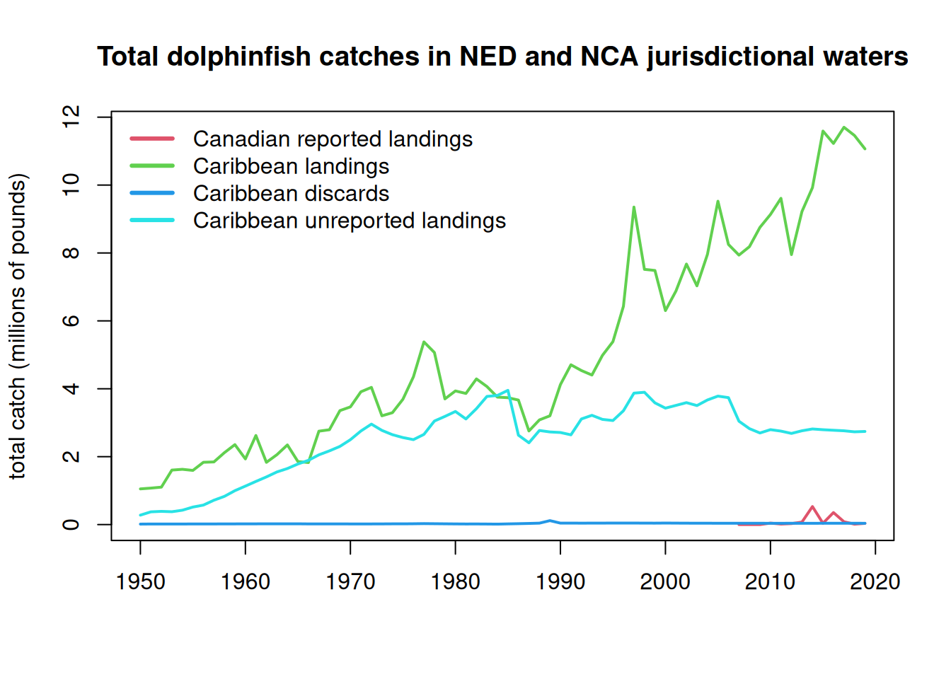
The catch from the Canadian EEZs is 100% landings, with no unreported data and no discards. In the WCA there are no reported discards, only unreported discards. Thus, we only need to separate out unreported discards and landings for the WCA.
# summarize the catch by year, area, discards/landings and reported/unreportedd$year <-factor(d$year, levels =1950:2019)dc <- d[which(d$reg =="Canadian EEZ"), ]dw <- d[which(d$reg =="Western Central Atlantic EEZs"), ]# verify proper identification of the erroneous Venezuelan Unknown Fishing Country catches bad <- dw[which(dw$area_name =="Venezuela"& dw$fishing_entity =="Unknown Fishing Country"), ]#dim(bad)bad_totals <-tapply(bad$lbs, bad$year, sum, na.rm = T)cbind(tail(bad_totals, 10), tail(removecatch, 10)) # the numbers match exactly
        [,1]    [,2]
2010      NA      NA
2011      NA      NA
2012      NA      NA
2013 1968566 1968566
2014 2759603 2759603
2015 4915156 4915156
2016 5112450 5112450
2017 6599737 6599737
2018 8236857 8236857
2019 7307245 7307245
# now remove those bad catches from the database prior to summarizing#dim(dw)dw <- dw[-which(dw$area_name =="Venezuela"& dw$fishing_entity =="Unknown Fishing Country"), ]#dim(dw)CAN <-tapply(dc$lbs, list(dc$year, dc$catch_type, dc$reporting_status), sum, na.rm = T)tail(CAN)
Note that the Caribbean unreported discards in the database are negligible (< 1%) and we exclude them from further analysis.
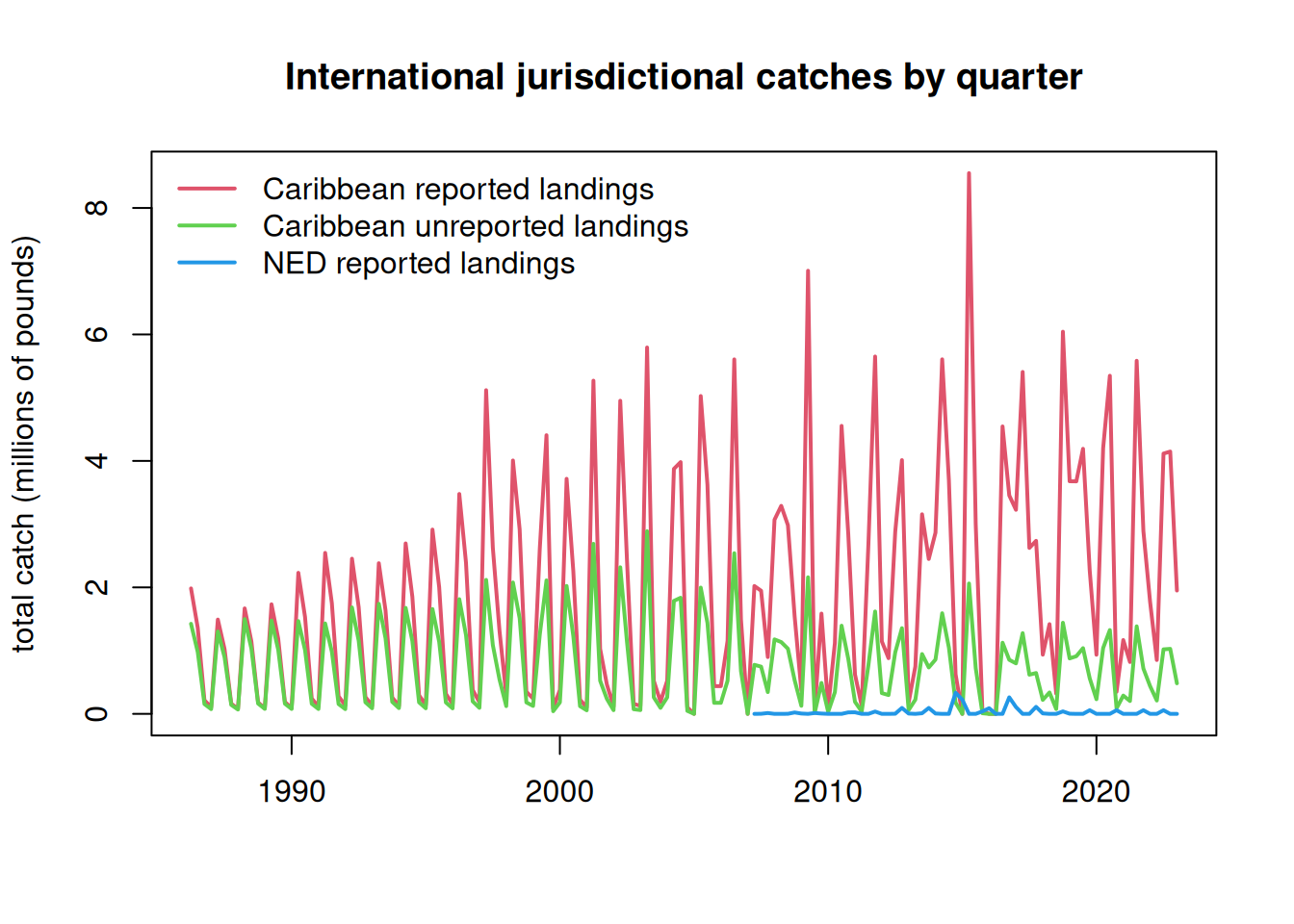
6.7 Distribute the territorial international catches across quarters of the year
The international catches are only reported as annual catches and do not have any month or season associated with them. However, the MSE operating model requires seasonal catches. Lacking other information on the seasonality of these fleets, we will assume that the fleet distribution of the U.S. pelagic longline is representative of the seasonality of the jurisdictional fleets. Now we parse the annual catches according to the seasonality of the U.S. fleet.
The pelagic longline logbook data is only available going back to 1997, but there are Caribbean catches extending back to the 1950s. To interpolate the seasonality for 1986 - 1996, we take the average seasonality of the oldest 10 years of logbook data (1997 - 2006) and use those averages for the unknown years.
At the time of analysis, the SAU database only contained catches to 2019, so we interpolated the 2019 values to cover years 2020 - 2022.
#par(mar = c(5, 10, 3, 1))#barplot(tapply(dw$lbs, dw$gear_type, sum, na.rm = T), horiz = T, las = 2)#barplot(tapply(dc$lbs, dc$gear_type, sum, na.rm = T), horiz = T, las = 2)# read in the percentage of the catch by area and year-quarter combinations from the U.S. PLLload("data/outputs/per_PLLcatch_by_area_yearquarter.RData") names(percatch[1, 1, ]) # matrix 2 == Caribbean, matrix 7 == NED (Atlantic Northwest)
[1] "NCA" "CAR" "FLK" "NCFL" "NNC" "VBM" "NED"
CAN <- CAN[which(rownames(CAN) >=1997)] # PLL data are only available from 1997 on CAN <-c(CAN, CAN[length(CAN)], CAN[length(CAN)], CAN[length(CAN)]) # interpolate 2019 catches for 2020-2022CANqrt <- percatch[, , 7] # create matrix for final catch datafor (i in1:ncol(percatch)) { CANqrt[, i] <- percatch[, i, 7] * CAN[i] }percatch_car <- percatch[, , 2] # create matrix for Caribbean percentagesint <-rowMeans(percatch_car[, 1:10]) # calculate the average seasonality using the oldest 10 years of logbook datapercatch_car <-cbind(matrix(rep(int, length(1986:1996)), nrow =4), percatch_car) # attach those 10-year averages to years 1986:1996colnames(percatch_car) <-1986:2022# full data frame for Caribbean seasonality 1986 - 2022CAR <- CAR[which(rownames(CAR) >=1986), ] # only need Caribbean data from 1986 on CAR <-rbind(CAR, CAR[nrow(CAR), ], CAR[nrow(CAR), ], CAR[nrow(CAR), ]) # interpolate 2019 catches for 2020-2022#dim(CAR)#dim(percatch_car)CARrep <- percatch_car # create matrices for final catch dataCARunr <- percatch_carfor (i in1:ncol(percatch_car)) { CARrep[, i] <- percatch_car[, i] * CAR[i, 1] CARunr[, i] <- percatch_car[, i] * CAR[i, 3]}# ensure sums are equal after parsingsum(CARrep); sum(CAR$landings)
[1] 286220280
[1] 286220280
sum(CARunr); sum(CAR$unreported)
[1] 112754888
[1] 112754888
sum(CAN, na.rm = T); sum(CANqrt, na.rm = T)
[1] 1328482
[1] 1328482
The Canada jurisdictional data need to be combined with the NED high seas data calculated in the previous section, because both of these are a component of the international catches in the NED area.
load("data/outputs/NED_year_quarter.RData")NEDtot <- NED + CANqrt# ensure sums are correctsum(NED, na.rm = T) +sum(CANqrt, na.rm = T); sum(NEDtot, na.rm = T)
[1] 1808855
[1] 1808855
NEDtot <- NEDtot[, !is.na(colSums(NEDtot))] # remove NA columns from CAN data# plot the parsed out data by year-quarteryrs <-sort(rep(as.numeric(colnames(CARrep)), 4))qrt <-rep(1:4, length(yrs)/4)yrs1 <-sort(rep(as.numeric(colnames(NEDtot)), 4))qrt1 <-rep(1:4, length(yrs1)/4)matplot(yrs + qrt/4, cbind(matrix(CARrep), matrix(CARunr))/10^6, lty =1, lwd =2, col =2:3, type ="l", main ="International jurisdictional catches by quarter", xlab ="", ylab ="total catch (millions of pounds)")lines(yrs1 + qrt1/4, as.numeric(matrix(NEDtot))/10^6, lwd =2, col =4)legend("topleft", c("Caribbean reported landings", "Caribbean unreported landings", "NED reported landings"), lwd =2, col =2:4, bty ="n")
Finally, we format the data in the format for input into the operating model.